Deep learning: logistic regression

Vitaly Vlasov

Lviv University

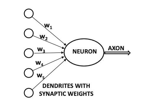
Neurons

Important

ANN \(\equiv\) Artificial Neural Network

Remember - Neurons, axons, dendrites.

Tip

Inputs to neurons are scaled with weight.

Weight is similar to a strength of synaptic connection.

Neurons

Neurons

Computation

ANN computes a function of the inputs by propagating the computed values from input neurons to output neurons, using weights as intermediate parameters.

Learning

Learning occurs by changing the weights. External stimuli are required for learning in bio-organisms, in case of ANNs they are provided by the training data.

Training

Training data contain input-output pairs. We compare predicted output with annotated output label from training data.

Neurons

Errors

Errors are comparison failures. These are similar to unpleasant feedback modifying synaptic strengths. Goal of changing weights - make predictions better.

Model generalizations

Ability to compute functions of unseen inputs accurately, even though given finite sets of input-output pairs.

Computation graph

Alternative view - computation graph.

When used in basic graph, NNs reduce to classical ML models.

• Least-squares regression
• logistic regression
• linear regression

Nodes compute based on inputs and weights.

Goal

Goal of NN: learn a function that relates inputs to outputs with the use of training examples.

Settings the edge weights is training.

Structure

Consider a simple case of \(d\) inputs and a single binary output. \[ (\overline{X}, y) - \text{training instance} \]

Feature variables: \[ \overline{X}=[x_1, \dots, x_d] \] Observed value: \(y \in {0,1}\), contained in target variable \(y\).

Objective

• learn the function \(f(\cdot)\), such that \(y=f_{\overline{W}}(\overline{X})\).

• minimize mismatch between \(y\) and \(f_{\overline{W}}(\overline{X})\). \(W\) - weight vector.

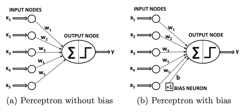
In case of perceptron, we compute a linear function: \[\begin{align*} &\hat{y}=f(\overline{X}) = sign\left\{\overline{W}^T \overline{X}^T\right\} = sign\left\{\sum\limits_{i=1}^d w_i x_i\right\} \end{align*}\] \(\hat{y}\) means value, not observed value \(y\).

Perceptron

A simplest NN.

Perceptron

We choose the basic form of the function, but strive to find some parameters.

• Sign is an activation function
• value of the node is also sometimes referred to as an activation.

Perceptron is a single-layer network, as input nodes are not counted.

Perceptron

How does perceptron learn? \[ \overline{W} := \overline{W} + \alpha(y-\hat{y})\overline{X}^T. \] So, in case when \(y \neq \hat{y}\), we can write it as \[ \overline{W} := \overline{W} + \alpha y \overline{X}^T. \]

Perceptron

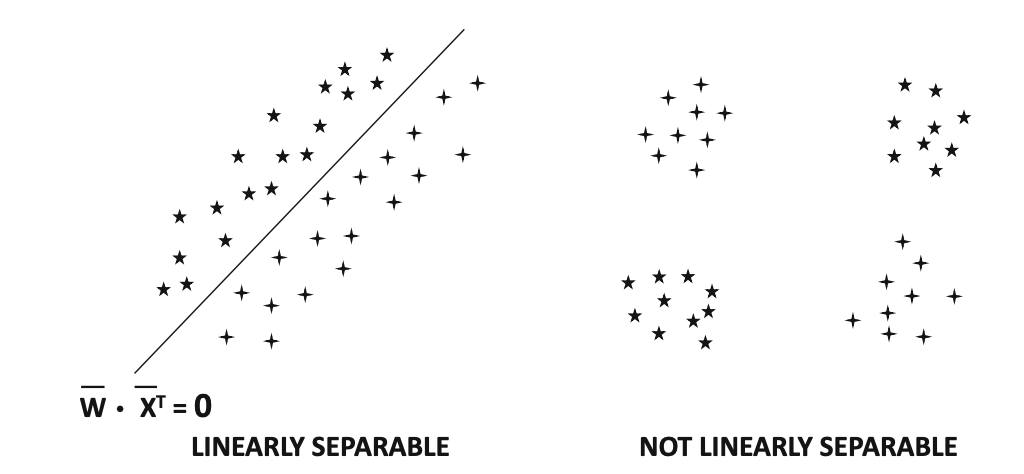
We can show that perceptron works when data are linearly separable by a hyperplane \(\overline{W}^T X = 0\).

Perceptron algorithm is not guaranteed to converge when data are not linearly separable.

Bias

Bias is needed when binary class distribution is imbalanced: \[ \overline{W}^T \cdot \sum_i \overline{X_i}^T \neq \sum_i y_i \] Bias can be incorporated by using a bias neuron.

Problems

In linearly separable data sets, a nonzero weight vector \(W\) exists in which the \(sign(\overline{W}^T X) = sign(y_i)\; \forall (\overline{X}_i,y_i)\).

However, the behavior of the perceptron algorithm for data that are not linearly separable is rather arbitrary.

Loss function

ML algorithms are loss optimization problems, where gradient descent updates are used to minimize the loss.

Original perceptron did not formally use a loss function.

Retrospectively we can introduce it as: \[ L_i \equiv \max\left\{-y_i(\overline{W}^T \overline{X_i}\right\} \]

Loss function

We differentiate: \[\begin{align*} &\dfrac{\partial L_i}{\partial \overline{W}} = \left[\dfrac{\partial L_i}{\partial w_1}, \dots, \dfrac{\partial L_i}{\partial w_d}\right] = \\ & = \begin{cases} -y_i \overline{X_i}, & \text{if } sign\{W^T X_i\} \neq y_i,\\ 0, & \text{otherwise} \end{cases} \end{align*}\]

Perceptron update

Negative of the vector is the direction of the fastest rate of loss reduction, hence perceptron update: \[\begin{align*} &\overline{W} := \overline{W} - \alpha\dfrac{\partial L_i}{\partial \overline{W}} = \overline{W} + \alpha y_i \overline{X_i}^T. \end{align*}\]

Activation functions

A network with weights \(\overline{W}\) and input \(\overline{X}\) will have a prediction of the form \[\begin{align*} &\hat{y}=\Phi\left( \overline{W}^T \overline{X}\right) \end{align*}\] where \(\Phi\) denotes activation function.

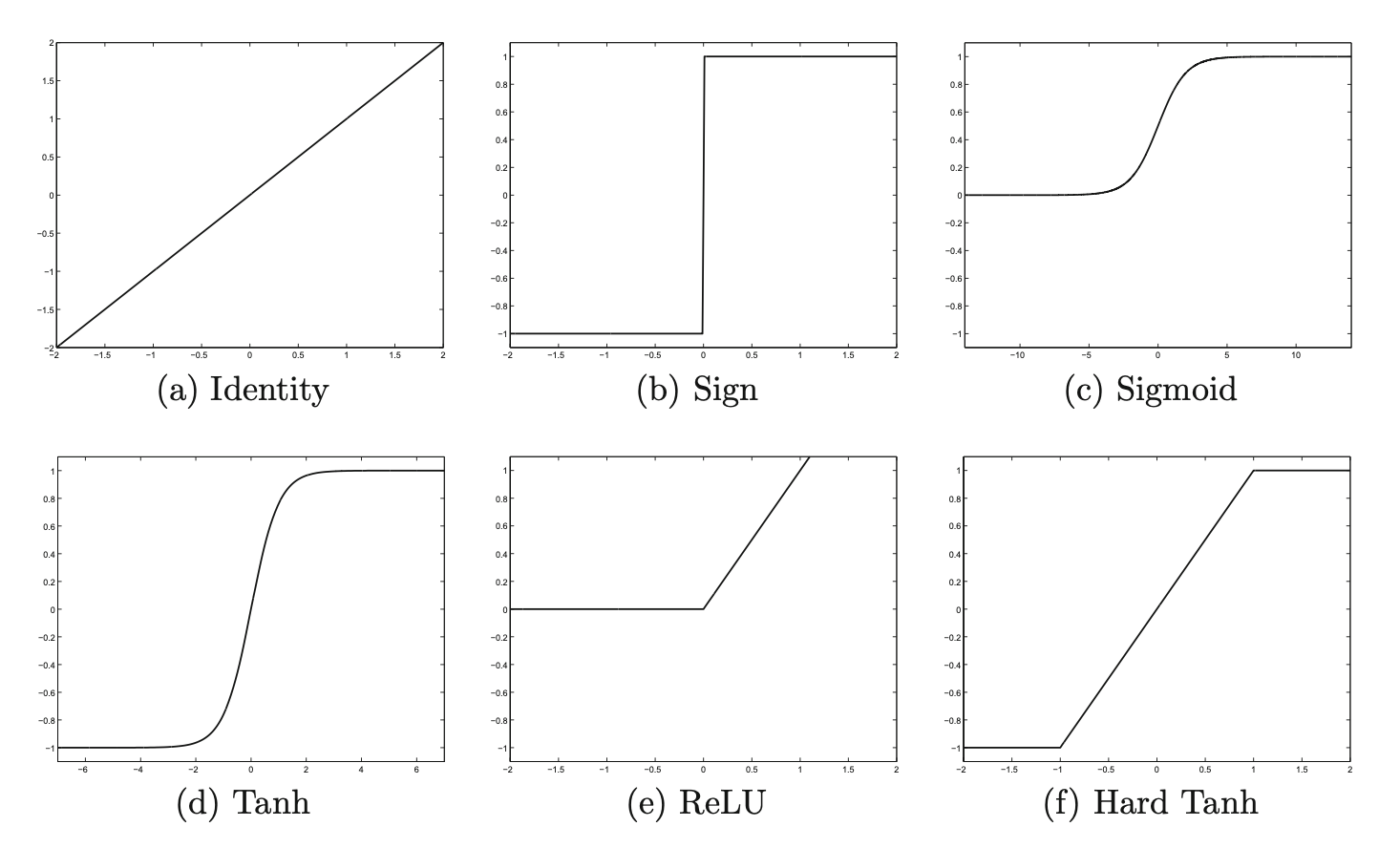
Activation functions

Identity aka linear activation

\[ \Phi(v) = v \]

Sign function

\[ \Phi(v) = sign(v) \]

Activation functions

Sigmoid function

\[ \Phi(v) = \dfrac{1}{1+e^{-v}} \]

tanh

\[ \Phi(v) = \dfrac{e^{2v}-1}{e^{2v}+1} \]

Activation functions

Actually, neuron computes two functions:

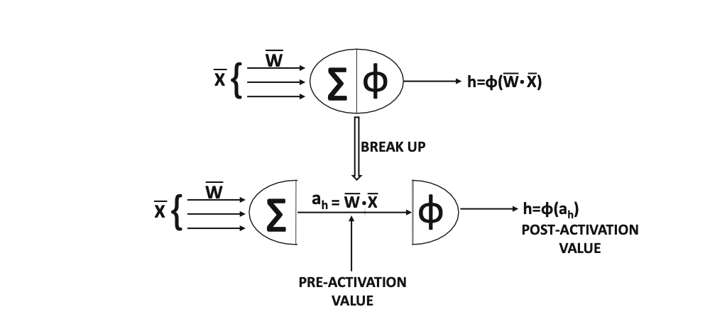
Activation functions

We have pre-activation value and post-activation value.

• pre-activation: linear transformation
• post-activation: nonlinear transformation

Activation functions

Activation functions

Activation functions

Two more functions that have become popular recently:

Rectified Linear Unit (ReLU)

\[ \Phi(v) = \max\left\{v, 0\right\} \]

Hard tanh

\[ \Phi(v) = \max\left\{\min\left[v, 1\right], -1 \right\} \]

Multiple activation fns

Activation functions

Properties:

• monotonic
• saturation at large values
• squashing

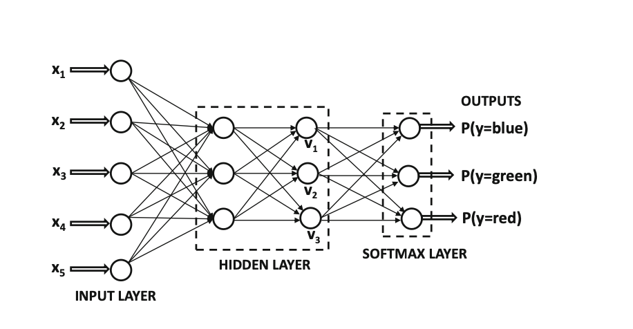
Softmax activation function

Used for k-way classification problems. Used in the output layer.

\[\begin{align*} &\Phi(v)_i = \dfrac{\exp(v_i)}{\sum\limits_{i=1}^k \exp(v_i)}. \end{align*}\]

Softmax layer converts real values to probabilities.

Softmax activation function

Loss functions

Least squares regression, numeric targets

\[\begin{align*} &L(\hat{y}, y) = (y-\hat{y})^2 \end{align*}\]

Logistic regression, binary targets

\[\begin{align*} &L(\hat{y}, y) = -\log \left|y/2 - 1/2 + \hat{y}\right|, \{-1,+1\} \end{align*}\]

Multinomial logistic regression, categorical targets

\[\begin{align*} &L(\hat{y}, y) = -\log (\hat{y}_r) \text{ - cross-entropy loss} \end{align*}\]

Multilayer networks

Multilayer networks

Suppose NN contains \(p_1, \dots, p_k\) units in each of its \(k\) layers.

Then column representations of these layers, denoted by \(\overline{h}_1, \dots, \overline{h}_k\), have \(p_1, \dots, p_k\) units.

• Weights between input layer and first hidden layer: matrix \(W_1\), sized \(p_1 \times d\).

• Weights between \(r\)-th layer and \(r+1\)-th layer: matrix \(W_r\) sized \(p_{r+1}\times p_r\).

Multilayer networks

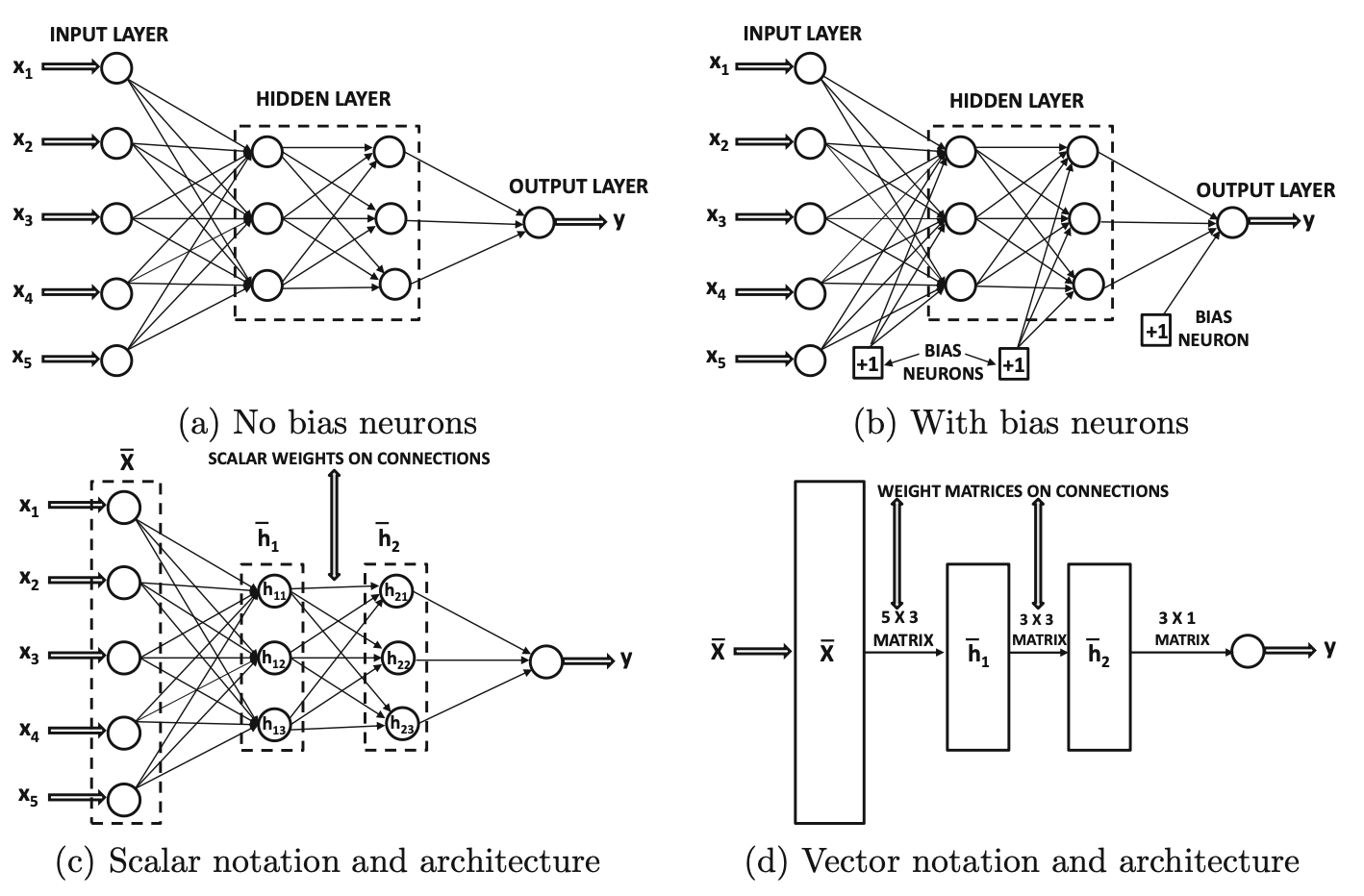
Multilayer networks

Therefore, a \(d\)-dimensional input vector \(\overline{x}\) is transformed into the outputs using these equations: \[\begin{align*} &\overline{h}_1 = \Phi(W_1^T x),\\ &\overline{h}_{p+1} = \Phi(W_{p+1}^T \overline{h}_p), \forall p \in \left\{1 \dots k-1 \right\} \\ &\overline{o} = \Phi(W_{k+1}^T \overline{h}_k) \end{align*}\] Activation functions operate on vectors and are applied element-wise.

Multilayer networks

Definition (Aggarwal)

A multilayer network computes a nested composition of parameterized multi-variate functions.

The overall function computed from the inputs to the outputs can be controlled very closely by the choice of parameters.

The notion of learning refers to the setting of the parameters to make the overall function consistent with observed input-output pairs.

Multilayer networks

Input-output function of NN is difficult to express explicitly. NN can also be called universal function approximators.

Universal approximation theorem

Given a family of neural networks, for each function \(\displaystyle f\) from a certain function space, there exists a sequence of neural networks \(\phi_1,\phi_2,\dots\) from the family, such that \(\phi_{n} \to f\) according to some criterion.

In other words, the family of neural networks is dense in the function space.

K. Hornik, M. Stinchcombe, and H. White. . Neural Networks, 2(5), pp. 359–366, 1989.

Nonlinear activation functions

Theorem. A multi-layer network that uses only the identity activation function in all its layers reduces to a single-layer network.

Proof. Consider a network containing \(k\) hidden layers, therefore containing a total of \((k+1)\) computational layers (including the output layer).

The corresponding \((k+1)\) weight matrices between successive layers are denoted by \(W_1 ...W_{k+1}\).

Nonlinear activation functions

Let:

• \(\overline{x}\) be the \(d\)-dimensional column vector corresponding to the input
• \(\overline{h_1},\dots,\overline{h_k}\) be the column vectors corresponding to the hidden layers
• and \(\overline{o}\) be the \(m\)-dimensional column vector corresponding to the output.

Nonlinear activation functions

Then, we have the following recurrence condition for multi-layer networks: \[\begin{align*} &\overline{h_1} = \Phi(W_1 x) = W_1 x,\\ &\overline{h}_{p+1} = \Phi(W_{p+1} \overline{h}_p) = W_{p+1}\overline{h}_p \;\; \forall p \in \left\{1 \dots k−1\right\}, \\ &\overline{o} = \Phi(W_{k+1} \overline{h}_k) = W_{k+1} \overline{h}_k. \end{align*}\]

Nonlinear activation functions

In all the cases above, the activation function \(\Phi(\cdot)\) has been set to the identity function. Then, by eliminating the hidden layer variables, we obtain the following: \[\begin{align*} &\overline{o} = W_{k+1}W_k \dots W_1 \overline{x} \end{align*}\] Denote \(W_{xo}=W_{k+1}W_k \dots W_1\).

Note

One can replace the matrix \(W_{k+1}W_k \dots W_1\) with the new \(d\times m\) matrix \(W_{xo}\), and learn the coefficients of \(W_{xo}\) instead of those of all the matrices \(W_1, W_2, \dots W_{k+1}\), without loss of expressivity.

Nonlinear activation functions

In other words, we have the following: \[\begin{align*} &\overline{o} = W_{xo} \overline{x} \end{align*}\] However, this condition is exactly identical to that of linear regression with multiple outputs. Therefore, a multilayer neural network with identity activations does not gain over a single-layer network in terms of expressivity.

Linearity observation

The composition of linear functions is always a linear function. The repeated composition of simple nonlinear functions can be a very complex nonlinear function.

Backpropagation

DAG Definition

A directed acyclic computational graph is a directed acyclic graph of nodes, where each node contains a variable. Edges might be associated with learnable parameters.

A variable in a node is either fixed externally (for input nodes with no incoming edges), or it is a computed as a function of the variables in the tail ends of edges incoming into the node and the learnable parameters on the incoming edges.

DAG is a more general version of NN.

Backpropagation

A computational graph evaluates compositions of functions.

A path of length 2 in a computational graph in which the function \(f(\cdot)\) follows \(g(\cdot)\) can be considered a composition function \(f(g(\cdot))\).

In case of sigmoid function: \[\begin{align*} &f(x) = g(x) = \dfrac{1}{1+e^{-x}} \\ &f(g(x)) = \dfrac{1}{1 + e^{\left[-\dfrac{1}{1+e^{-x}}\right]}} \end{align*}\]

Backpropagation

Important

The inability to easily express the optimization function in closed form in terms of the edge-specific parameters (as is common in all machine learning problems) causes difficulties in computing the derivatives needed for gradient descent.

Example

For example, if we have a computational graph which has 10 layers, and 2 nodes per layer, the overall composition function would have \(2^{10}\) nested “terms”.

Backpropagation

1. Derivatives of the output with respect to various variables in the computational graph are related to one another with the use of the chain rule of differential calculus.
2. Therefore, the chain rule of differential calculus needs to be applied repeatedly to update derivatives of the output with respect to the variables in the computational graph.
3. This approach is referred to as the backpropagation algorithm, because the derivatives of the output with respect to the variables close to the output are simpler to compute (and are therefore computed first while propagating them backwards towards the inputs).

Derivatives are computed numerically, not algebraically.

Backpropagation

Forward phase

• Use the attribute values from the input portion of a training data point to fix the values in the input nodes.
• Select a node for which the values in all incoming nodes have already been computed and apply the node-specific function to also compute its variable.
• Repeat the process until the values in all nodes (including the output nodes) have been computed.
• Compute loss value if the computed and observed values mismatch.

Backpropagation

Backward phase

• Compute the gradient of the loss with respect to the weights on the edges.
• Derivatives of the loss with respect to weights near the output (where the loss function is computed) are easier to compute and are computed first.
• The derivatives become increasingly complex as we move towards edge weights away from the output (in the backwards direction) and the chain rule is used repeatedly to compute them.
• Update the weights in the negative direction of the gradient.

Single cycle through all training points is an epoch.

Logistic Regression as a Neural Network

Inputs

Logistic regression is an algorithm for binary classification.

\(x \in \mathbb{R}^{n_x}, y \in \{0,1\}\).

\(\left\{(x^{(1)},y^{(1)}), ...(x^{(m)}, y^{(m)})\right\}\)- \(m\) training examples.

\(X\) matrix - \(m\) columns and \(n_x\) rows.

\[\begin{align*} &X = \begin{bmatrix} \vdots & \vdots & \dots & \vdots \\ x^{(1)} & x^{(2)} & \dots & x^{(m)} \\ \vdots & \vdots & \dots & \vdots \end{bmatrix} \end{align*}\]

\[ Y = \left[y^{(1)}, y^{(2)}, \dots, y^{(m})\right] \]

Logistic Regression

\(X \in \mathbb{R}^{n_x,m}\).

Using Numpy syntax:

X.shape = (n_x,m).

\(Y \in \mathbb{R}^{1,m}\).

Using Numpy syntax:

Y.shape = (1,m).

Logistic Regression

Goal

We will strive to maximize \(\hat{y} = P(y=1 | x)\), where \(x \in \mathbb{R}^{n_x}\).

Obviously, \(0 \leq \hat{y} \leq 1\).

Important

If doing linear regresssion, we can try \[ \hat{y}=w^T x + b. \]

But for logistic regression, we do \[ \hat{y}=\sigma(w^T x + b)$, \; \text{where }\; \sigma=\dfrac{1}{1+e^{-z}}. \]

Parameters

Input

\[ w \in \mathbb{R}^{n_x},\\ b \in \mathbb{R}. \]

Output

\[ \hat{y} = \sigma\left( w^T x + b\right), \]

\[ z \equiv w^T x + b. \]

\(w\) - weights, \(b\) - bias term (intercept)

Graphs

\(\sigma=\dfrac{1}{1+e^{-z}}\).

Loss function

For every \(\left\{(x^{(1)},y^{(1)}), ...(x^{(m)}, y^{(m)})\right\}\), we want to find \(\hat{y}^{(i)} \approx y^{(i)}\). \[\begin{align*} &\hat{y}^{(i)} = \sigma\left(w^T x^{(i)} + b\right) \end{align*}\] We have to define a loss (error) function - this will estimate our model.

Loss function

Quadratic

\[ L(\hat{y}, y) = \dfrac{1}{2}\left(\hat{y}-y)\right)^2. \]

Log

\[ L(\hat{y}, y) = -\left((y\log(\hat{y}) + (1 - y)\log(1 - \hat{y}))\right). \]

Cost function

Why does it work well?

Consider \(y=0\) and \(y=1\).

\[\begin{align*} &y=1: P(y | x) = \hat{y},\\ &y=0: P(y | x) = 1-\hat{y} \end{align*}\]

We select \(P(y|x) = \hat{y}^y(1-\hat{y})^{(1-y)}\).

\[ \log P(y|x) = y\log(\hat{y}) + (1-y)\log(1-\hat{y}) = -L(\hat{y}, y). \]

\[\begin{align*} y=1:& L(\hat{y},y) = -\log(\hat{y}),\\ y=0:& L(\hat{y},y) = -\log(1-\hat{y}) \end{align*}\]

Cost function

Cost function show how well we’re doing across the whole training set: \[\begin{align*} &J(w, b) = \dfrac{1}{m} \sum\limits_{i=1}^m L(\hat{y}^{(i)}, y^{(i)}) = \\ & = -\dfrac{1}{m} \sum\limits_{i=1}^m \left[y\log(\hat{y}) + (1 - y)\log(1 - \hat{y})\right]. \end{align*}\]

Cost function

On \(m\) examples: \[\begin{align*} &\log P(m \dots) = \log \prod_{i=1}^m P(y^{(i)} | x^{(i)}) = \\ & = \sum\limits_{i=1}^m \log P(y^{(i)} | x^{(i)}) = -\sum\limits_{i=1}^m L(\hat{y}^{(i)}, y^{(i)}). \end{align*}\]

Gradient descent

Problem

Minimization problem: find \(w,b\) that minimize \(J(w,b)\).

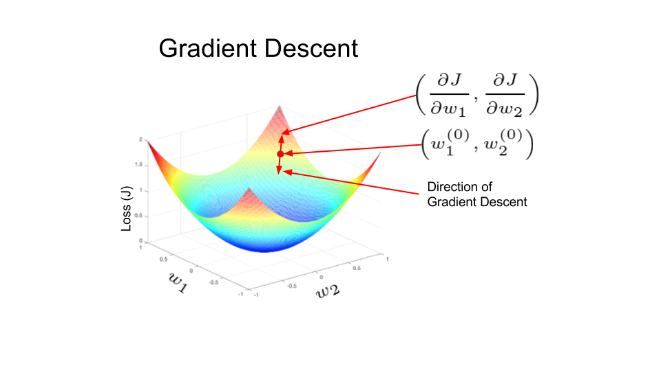
Gradient descent

• We use \(J(w,b)\) because it is convex.
• We pick an initial point - anything might do, e.g. 0.
• Then we take steps in the direction of steepest descent.

\[ w := w - \alpha \frac{d J(w,b)}{dw}, \\ b := b - \alpha \frac{d J(w,b)}{db} \]

\(\alpha\) - learning rate

Gradient descent

• forward pass: compute output
• backward pass: compute derivatives

Logistic Regression Gradient Descent

\[\begin{align*} &z = w^T x + b ,\\ &a \equiv \hat{y} = \sigma(z),\\ &L(a,y) = -\left[y\log(a) + (1 - y)\log(1 - a)\right]. \end{align*}\]

So, for \(n_x=2\) we have a computation graph:

\((x_1,x_2,w_1,w_2,b)\) \(\rightarrow\) \(z =w_1 x_1+w_2 x_2 + b\) \(\rightarrow\) \(\hat{y}=a=\sigma(z)\) \(\rightarrow\) \(L(a,y)\).

Computation graph

Let’s compute the derivative for \(L\) by a: \[\begin{align*} &\frac{dL}{da} = -\dfrac{y}{a} + \dfrac{1-y}{1-a},\\ &\frac{da}{dz} = a(1-a). \end{align*}\]

Computation graph

After computing, we’ll have \[\begin{align*} &dz \equiv \dfrac{dL}{dz} = \dfrac{dL}{da}\dfrac{da}{dz} = a-y,\\ &dw_1 \equiv \frac{dL}{dw_1} = x_1 dz,\\ &dw_2 \equiv \frac{dL}{dw_2} = x_2 dz, \\ &db \equiv \frac{dL}{db} = dz. \end{align*}\]

Logistic Regression Gradient Descent

GD steps are computed via \[\begin{align*} &w_1 := w_1 - \alpha \frac{dL}{dw_1},\\ &w_2 := w_2 - \alpha \frac{dL}{dw_2},\\ &b := b - \alpha \frac{dL}{db}. \end{align*}\]

Logistic Regression Gradient Descent

Consider now \(m\) examples in the training set.

Let’s recall the definition of the cost function: \[\begin{align*} &J(w,b) = \dfrac{1}{m}\sum\limits_{i=1}^{m} L(a^{(i)}, y^{(i)}, \\ &a^{(i)} = \hat{y}^{(i)}=\sigma(w^T x^{(i)} + b). \end{align*}\] And also \[ \frac{dJ}{dw_1} = \frac{1}{m}\sum\limits_{i=1}^{m}\frac{dL(a^{(i)}, y^{(i)})}{dw_1}. \]

Logistic Regression Gradient Descent

Let’s implement the algorithm. First, initialize \[ J=0,\\ dw_1=0,\\ dw_2=0,\\ db=0 \]

Logistic Regression Gradient Descent

for i=1 to m \[\begin{align*} &z^{(i)} = w^T x^{(i)} + b, \\ &a^{(i)} = \sigma(z^{(i)}), \\ &J += -\left[y^{(i)} \log a^{(i)} + (1-y^{(i)}) \log(1-a^{(i)})\right], \\ &dz^{(i)} = a^{(i)} - y^{(i)}, \\ &dw_1 += x_1^{(i)} dz^{(i)},\\ &dw_2 += x_2^{(i)} dz^{(i)},\\ &db += dz^{(i)}. \end{align*}\]

Logistic Regression Gradient Descent

Then compute averages:

\[ J = \dfrac{J}{m}, \\ dw_1 = \dfrac{dw_1}{m}, \; dw_2 = \dfrac{dw_2}{m}, \\ db = \dfrac{db}{m}. \]

Note that \(dw_i\) don’t have a superscript - we use them as accumulators. (In this example feature count \(n_x=2\))

GD step

\[ w_1 := w_1 - \alpha dw_1,\\ w_2 := w_2 - \alpha dw_2,\\ b := b - \alpha db. \]

Vectorization

We only have 2 features \(w_1\) and \(w_2\), so we don’t have an extra for loop. Turns out that for loops have a detrimental impact on performance.

Vectorization techniques exist for this purpose - getting rid of for loops.

Example

We have to compute \(z=w^T x + b\), where \(w,x \in \mathbb{R}^{n_x}\), and for this we can naturally use a for loop.

A vectorized Python command is

z = np.dot(w,x)+b

Vectorization

Programming guideline - avoid explicit for loops. \[\begin{align*} &u = Av,\\ &u_i = \sum_j\limits A_{ij} v_j \end{align*}\] To be replaced by

u = np.dot(A, v)

Numpy impl: https://numpy.org/doc/1.21/reference/simd/simd-optimizations.html

Vectorization

Another example. Let’s say we have a vector \[\begin{align*} &v = \begin{bmatrix} v_1 \\ \vdots \\ v_n \end{bmatrix}, u = \begin{bmatrix} e^{v_1},\\ \vdots \\ e^{v_n} \end{bmatrix} \end{align*}\] A code listing is

import numpy as np
u = np.exp(v)

So we can modify the above code to get rid of for loops (except for the one for \(m\)).

Vectorizing logistic regression

Let’s examine the forward propagation step of LR. \[\begin{align*} &z^{(1)} = w^T x^{(1)} + b,\\ &a^{(1)} = \sigma(z^{(1)}), \end{align*}\]

\[\begin{align*} &z^{(2)} = w^T x^{(2)} + b,\\ &a^{(2)} = \sigma(z^{(2)}). \end{align*}\]

Vectorizing logistic regression

Let’s recall what have we defined as our learning matrix: \[ X = \begin{bmatrix} \vdots & \vdots & \dots & \vdots \\ x^{(1)} & x^{(2)} & \dots & x^{(m)} \\ \vdots & \vdots & \dots & \vdots \end{bmatrix} \]

Vectorizing logistic regression

Next \[ Z = [z^{(1)}, \dots, z^{(m)}] = w^T X + [b, b, \dots, b] =\\ = [w^T x^{(1)}+b, \dots, w^T x^{(m)}+b]. \]

\[ A = \left[a^{(1)}, \dots, a^{(m)}\right] = \sigma\left(Z\right) \]

  z = np.dot(w.T, x) + b

\(b\) is a raw number, Python will automatically take care of expanding it into a vector - this is called broadcasting.

Vectorizing logistic regression

Earlier on, we computed \[\begin{align*} &dz^{(1)} = a^{(1)} - y^{(1)}, dz^{(2)} = a^{(2)} - y^{(2)}, \dots \end{align*}\]

We now define \[\begin{align*} &Y = [y^{(1)}, \dots, y^{(m)}],\\ &dZ = [dz^{(1)}, \dots, dz^{(m)}] =\\ &= A-Y = [a^{(1)}-y^{(1)}, \dots, a^{(m)}-y^{(m)}] \end{align*}\]

Vectorizing logistic regression

For \(db\) we have \[\begin{align*} &db = \frac{1}{m}np.sum(dZ),\\ &dw = \frac{1}{m}X dZ^T = \\ & \frac{1}{m}\begin{bmatrix} \vdots & & \vdots \\ x^{(1)} & \dots & x^{(m)} \\ \vdots & & \vdots \\ \end{bmatrix} \begin{bmatrix} dz^{(1)} \\ \vdots\\ dz^{(m)} \end{bmatrix} = \\ & = \frac{1}{m}\left[x^{(1)}dz^{(1)} + \dots +x^{(m)}dz^{(m)}\right]. \end{align*}\]

Vectorizing logistic regression

Now we can go back to the backward propagation algorithm again.

Multiple iterations of GD will still require a for loop.

for it in range(m):
  Z = np.dot(w.T, X) + B
  A = sigma(Z)
  dZ = A-Y
  dw = 1/m X * dZ.T
  db = 1/m np.sum(dZ)
  w := w - alpha * dw
  b := b - alpha * db