Transformers 1
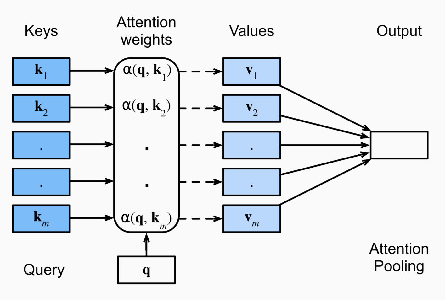
Attention
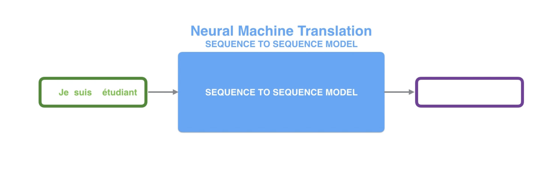
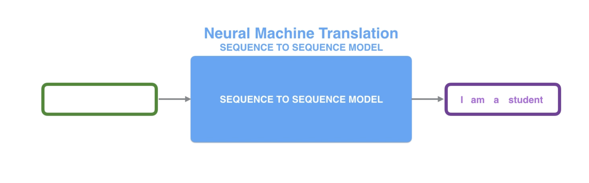
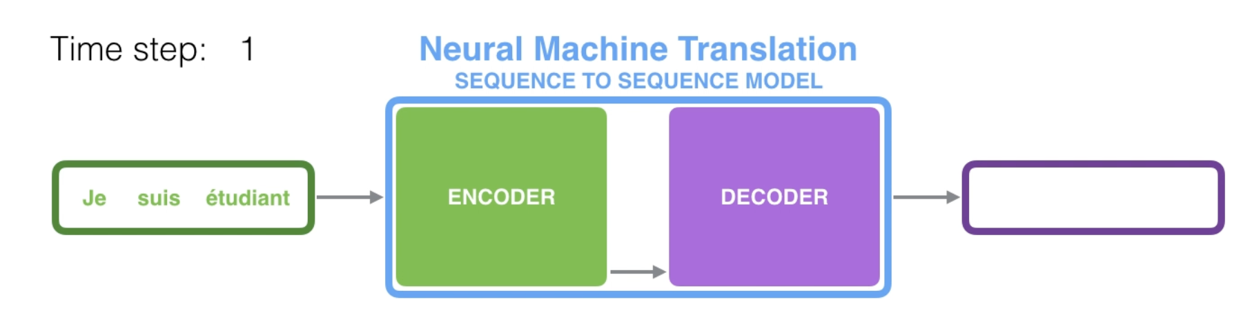
seq2seq
seq2seq
seq2seq
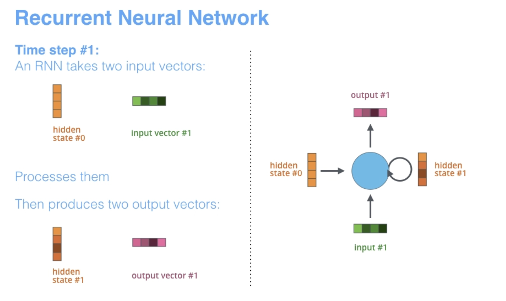
RNN takes two inputs: an input (one word from the input sentence) and a hidden state.
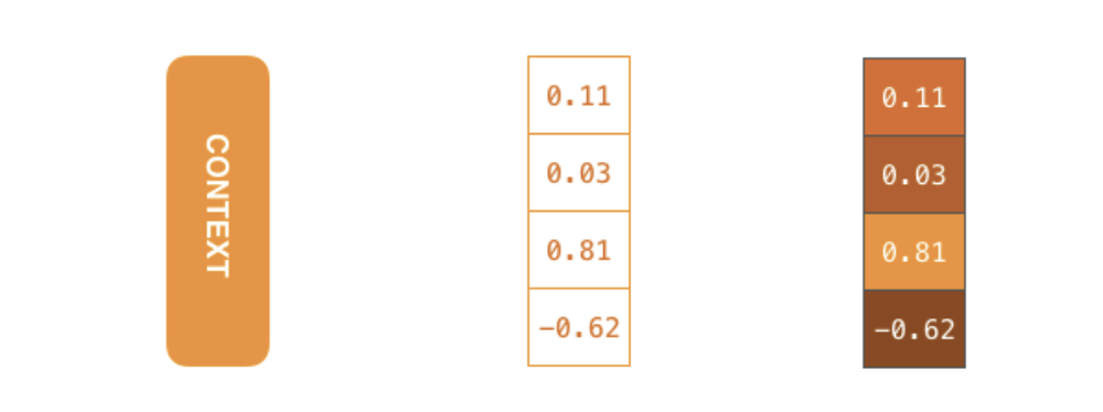
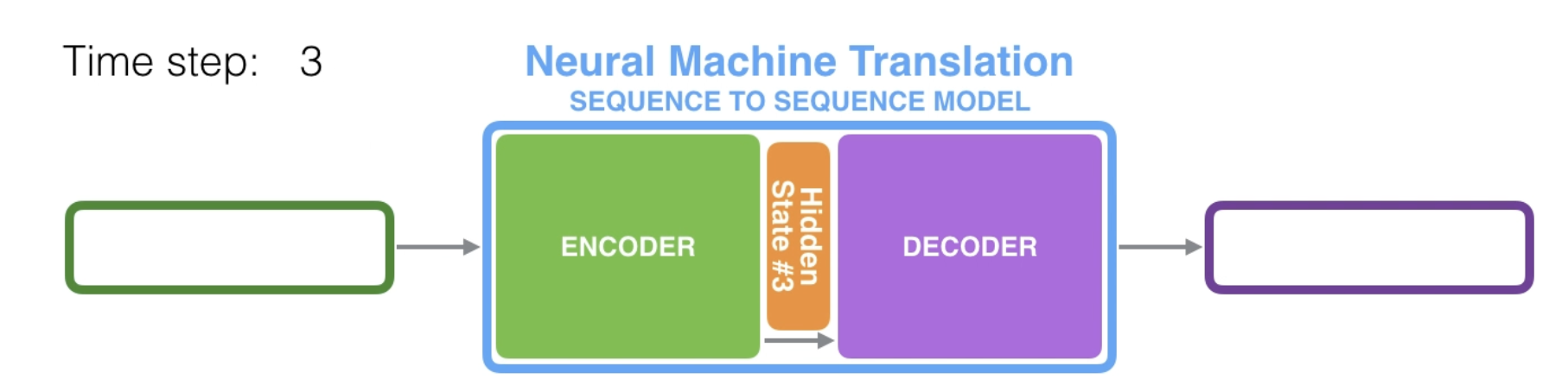
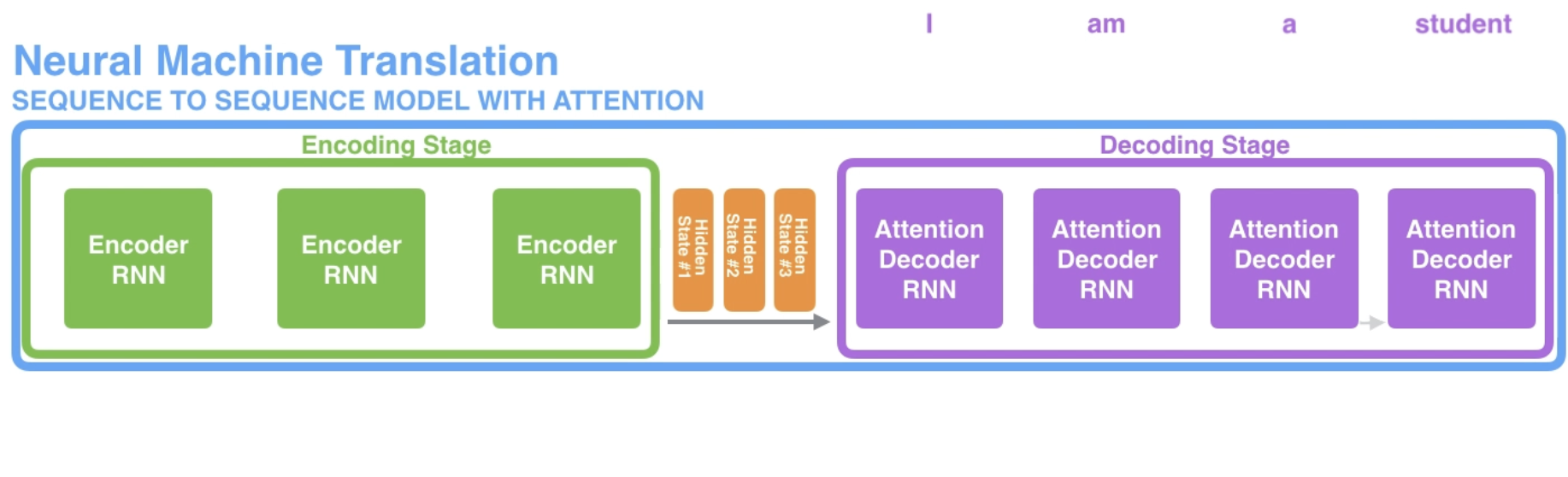
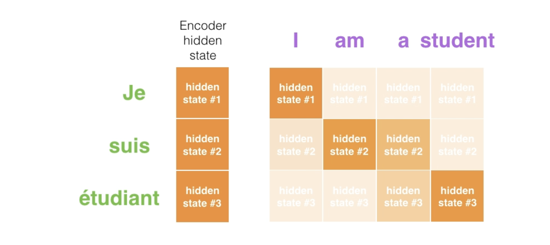
Context: You can set the size of the context vector when you set up your model. It is basically the number of hidden units in the encoder RNN. These visualizations show a vector of size 4, but in real world applications the context vector would be of a size like 256, 512, or 1024.
seq2seq


seq2seq
seq2seq
seq2seq
Unrolled view
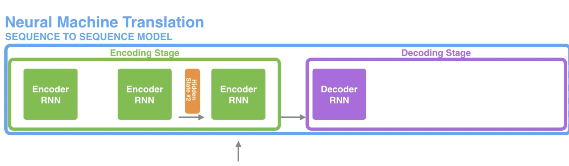
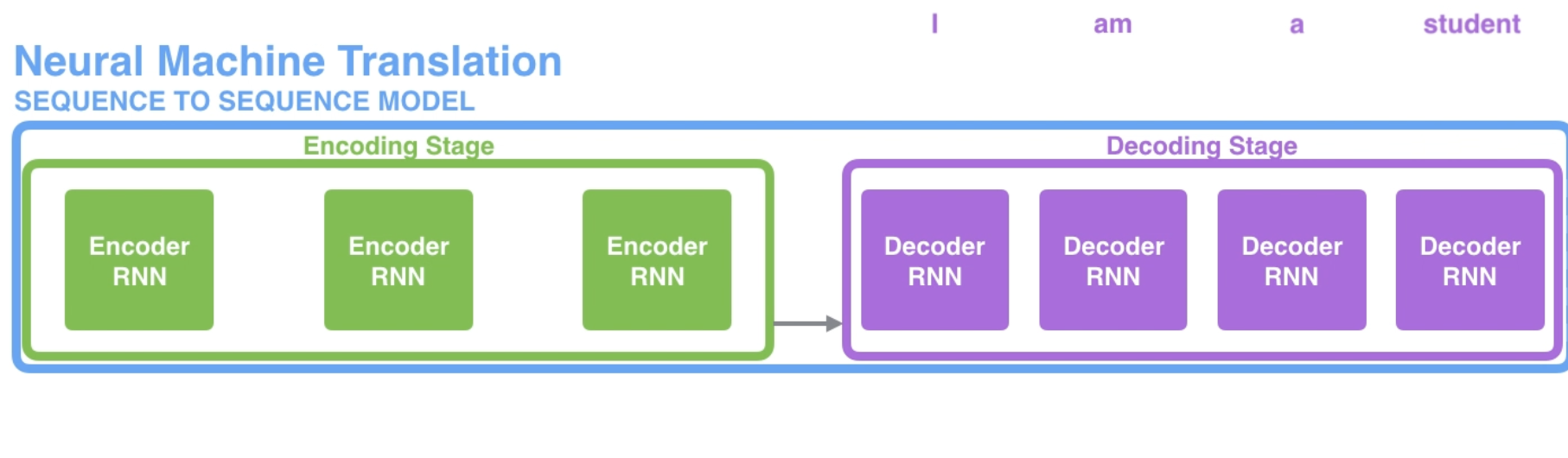
seq2seq
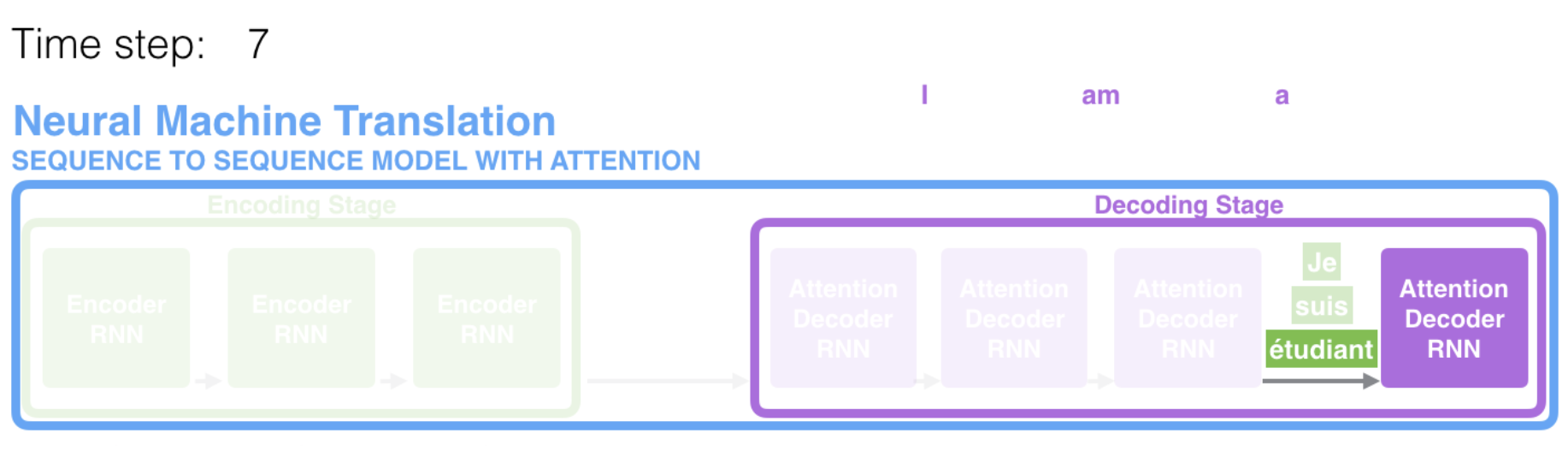
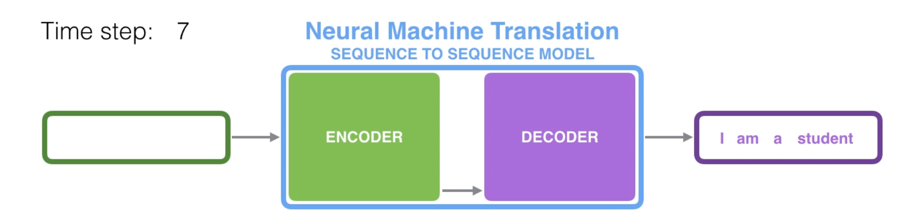
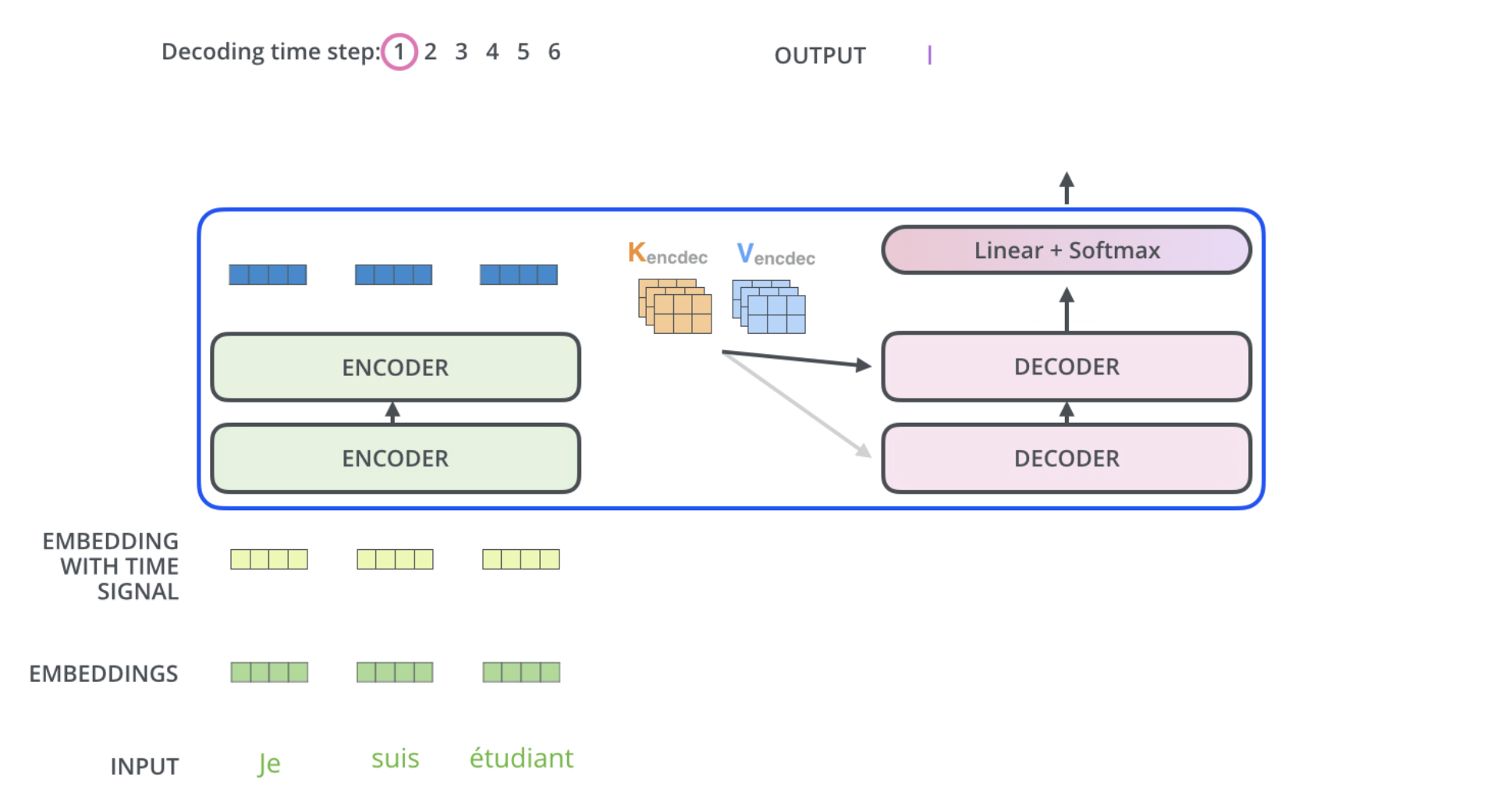
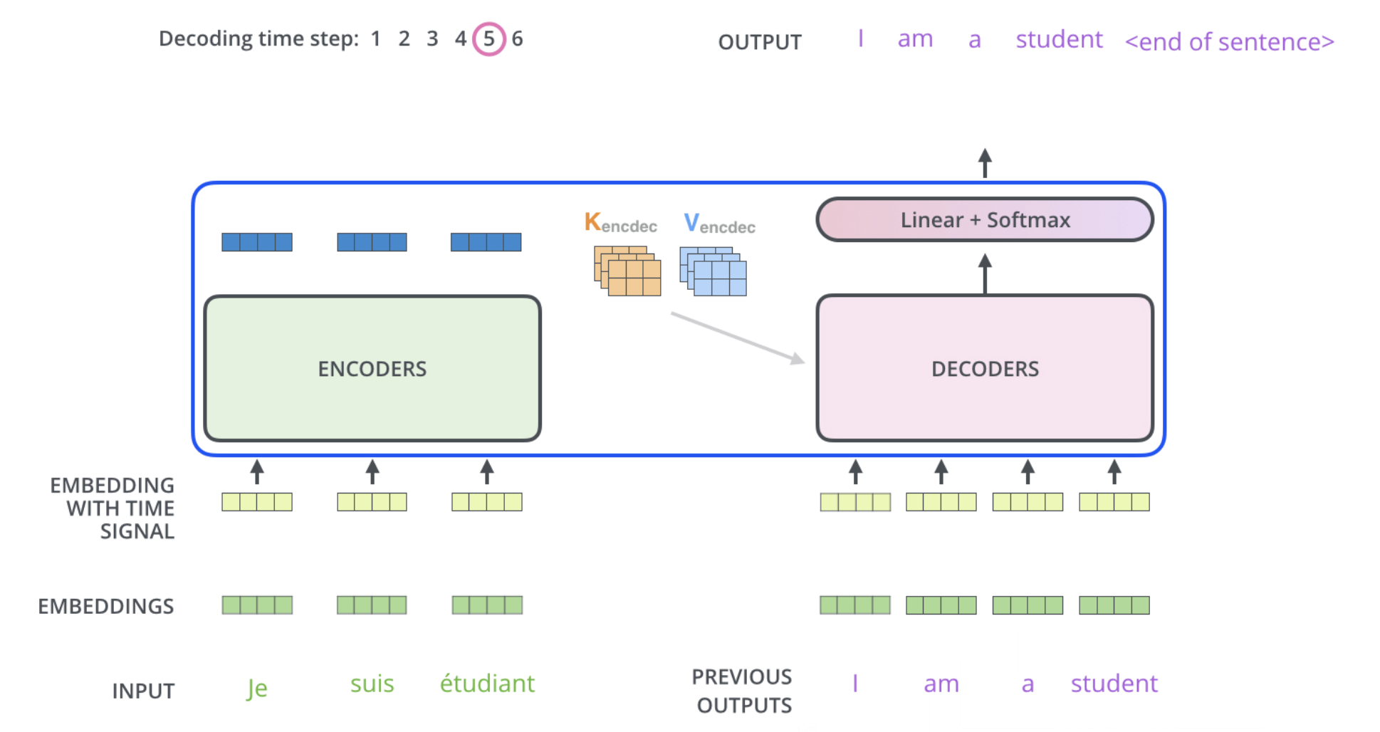
At time step 7, the attention mechanism enables the decoder to focus on the word “étudiant” (“student” in french) before it generates the English translation.
seq2seq
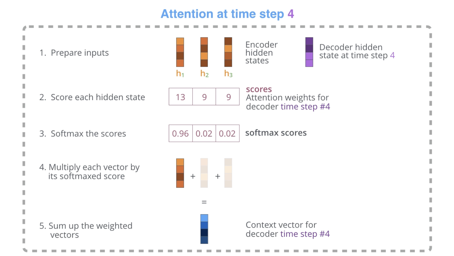
Illustrated
seq2seq
seq2seq
seq2seq
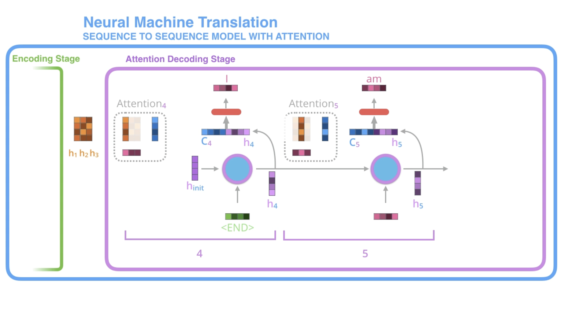
Another way
seq2seq
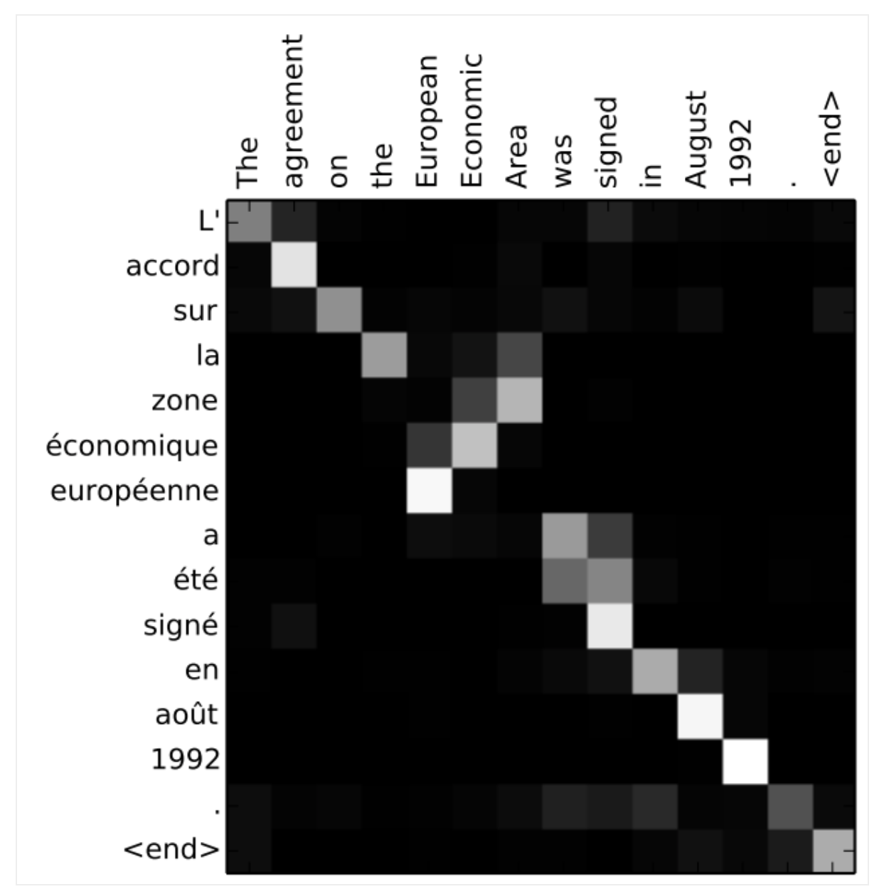
Model learns how to align words (example from paper).
Transformers
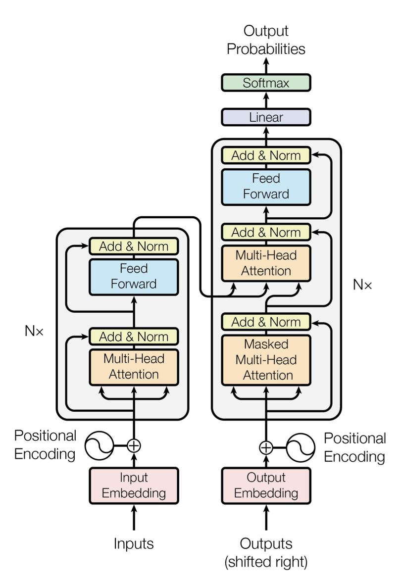
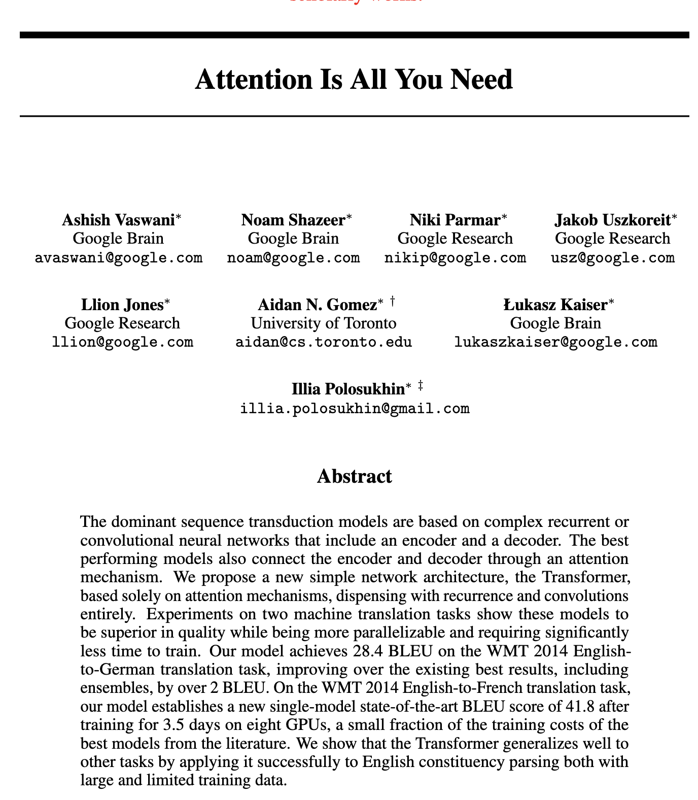
Attention is all you need (2017)
Transformers
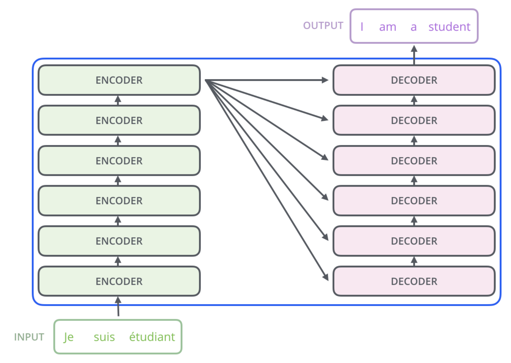
Compared to seq2seq, performance is improved!
Transformers
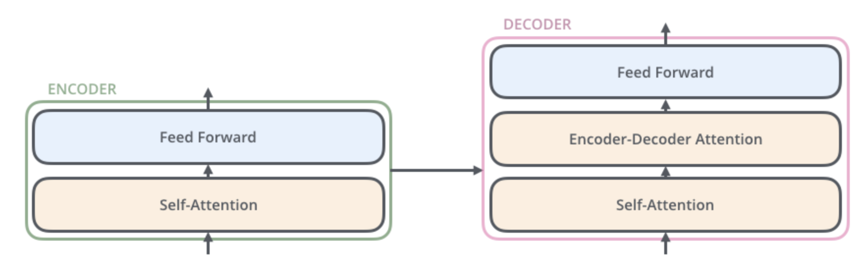
Encoder and decoder structure.
Transformers
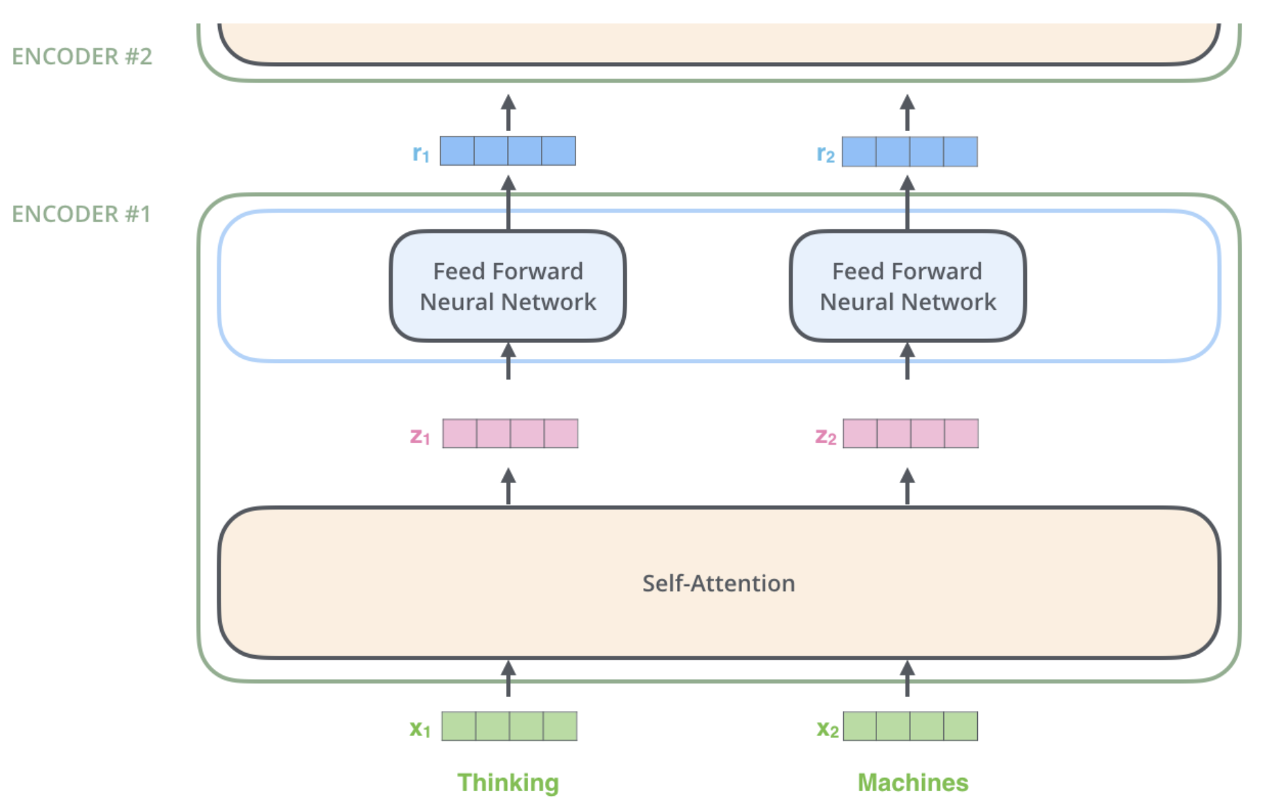
A key property of the Transformer: the word in each position flows through its own path in the encoder. There are dependencies between these paths in the self-attention layer. The feed-forward layer does not have those dependencies, however, and thus the various paths can be executed in parallel while flowing through the feed-forward layer.
Transformers
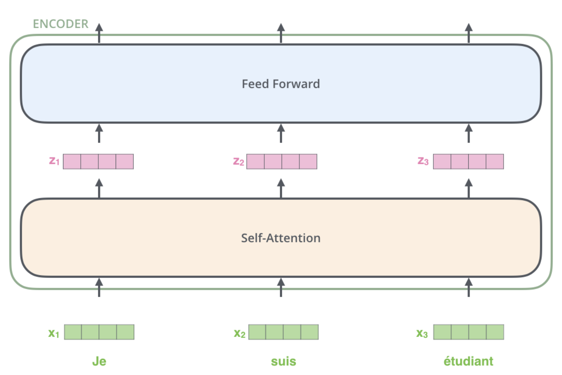
The word at each position passes through a self-attention process. Then, they each pass through a FFNN.
Transformers
Transformers
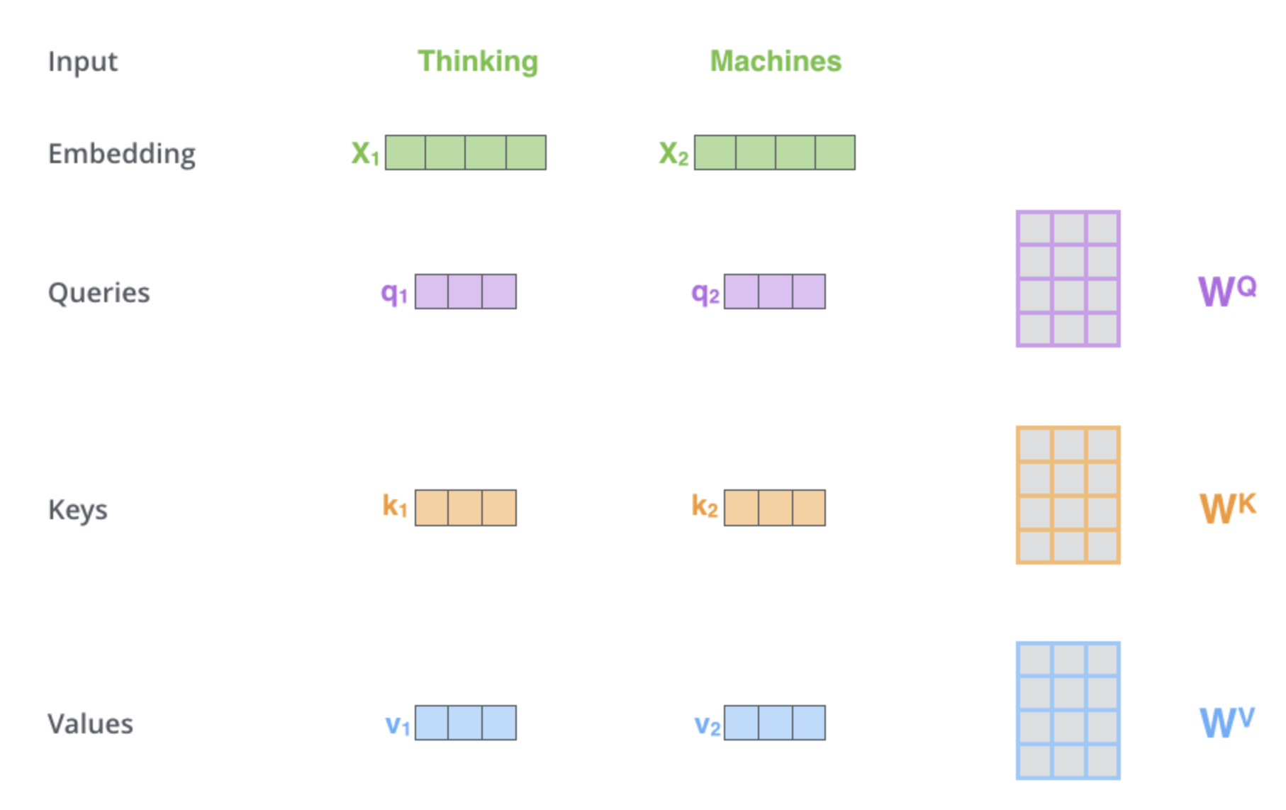
How is self-attention calculated?
- Create 3 vectors (Query, Key, Value) from each input embedding.
Transformers
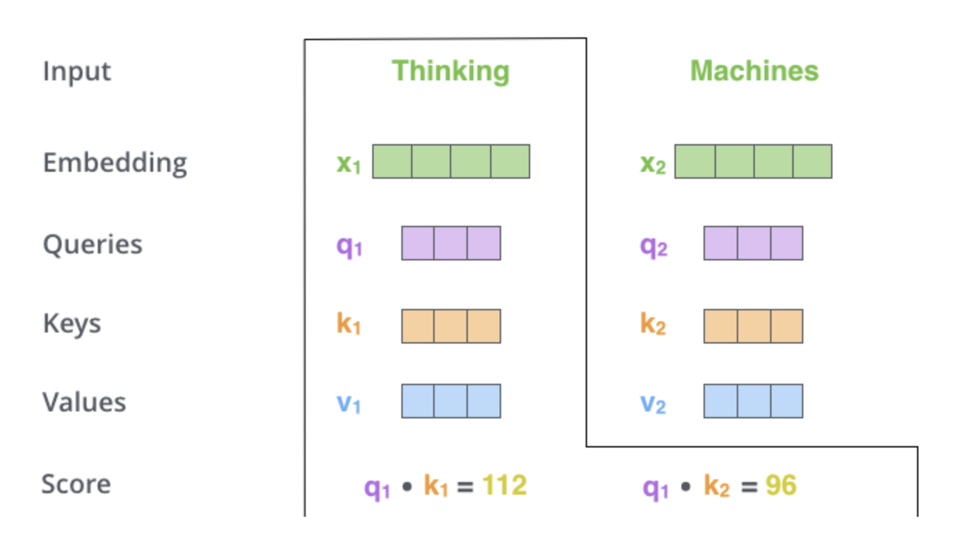
How is self-attention calculated?
- Calculate score. The score is calculated by taking the dot product of the query vector with the key vector of the respective word we’re scoring.
Transformers
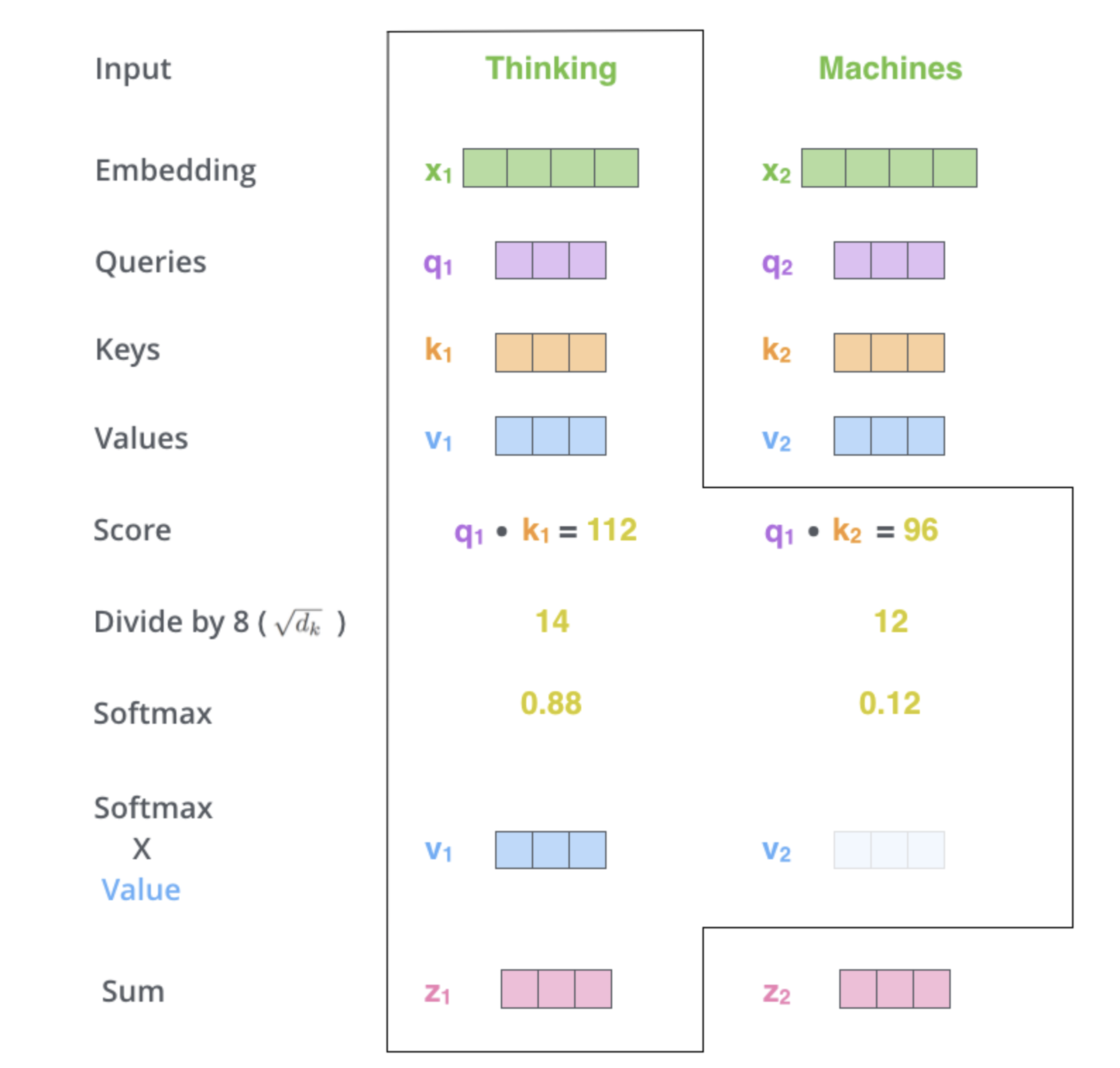
How is self-attention calculated?
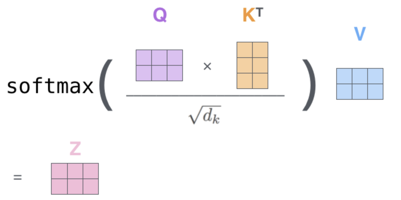
Divide by \(\sqrt{d_k}\).
Normalize via softmax.

Transformers
Transformers
Matrix calculation
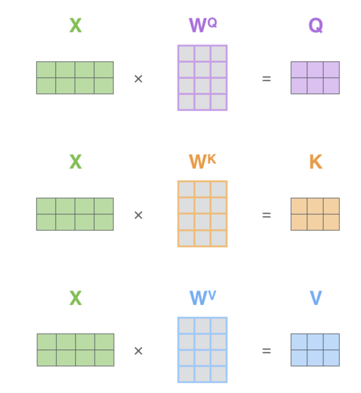
Transformers
Matrix calculation
Transformers
Transformers
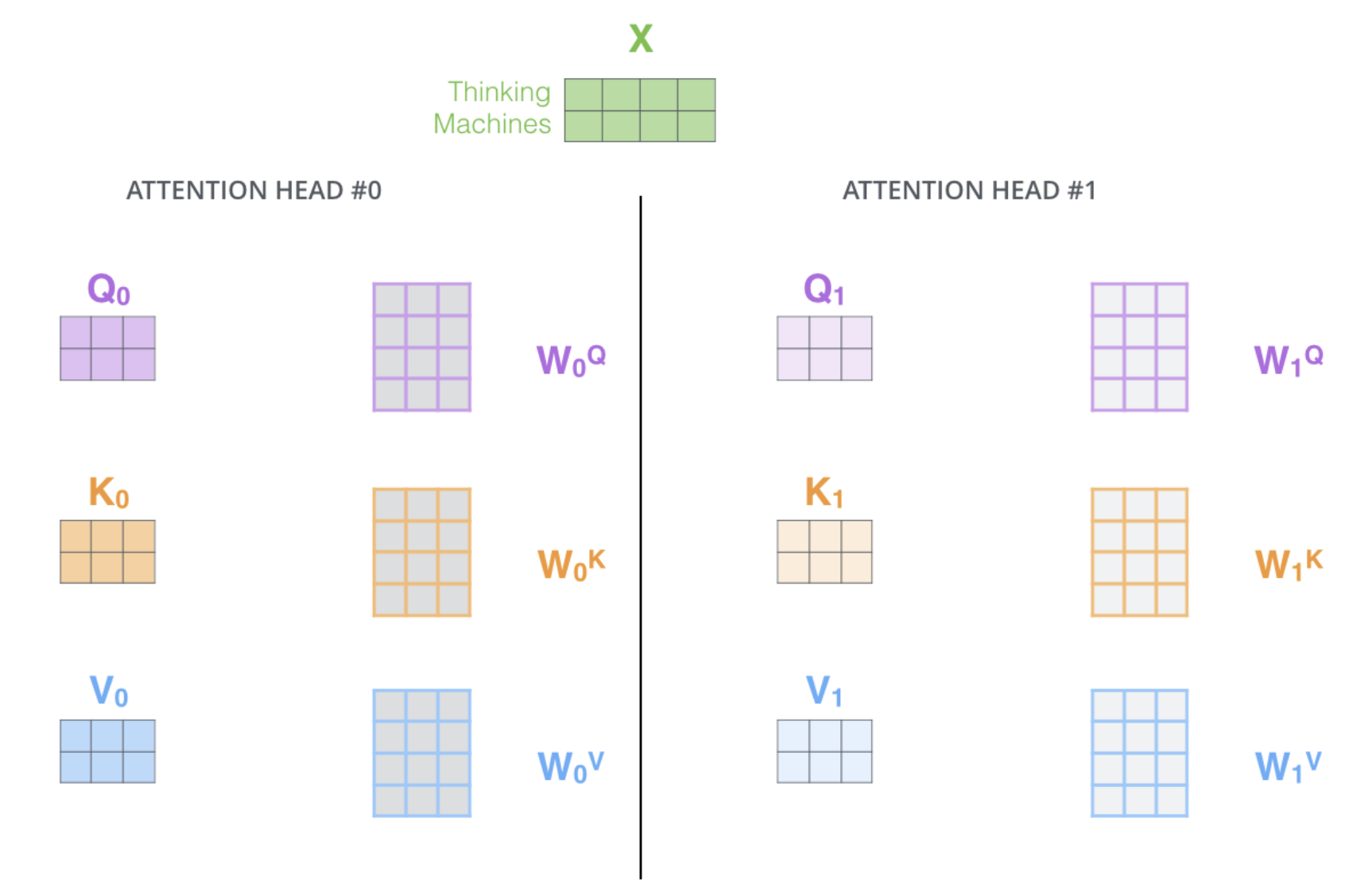
Calculating e.g. 8 times: 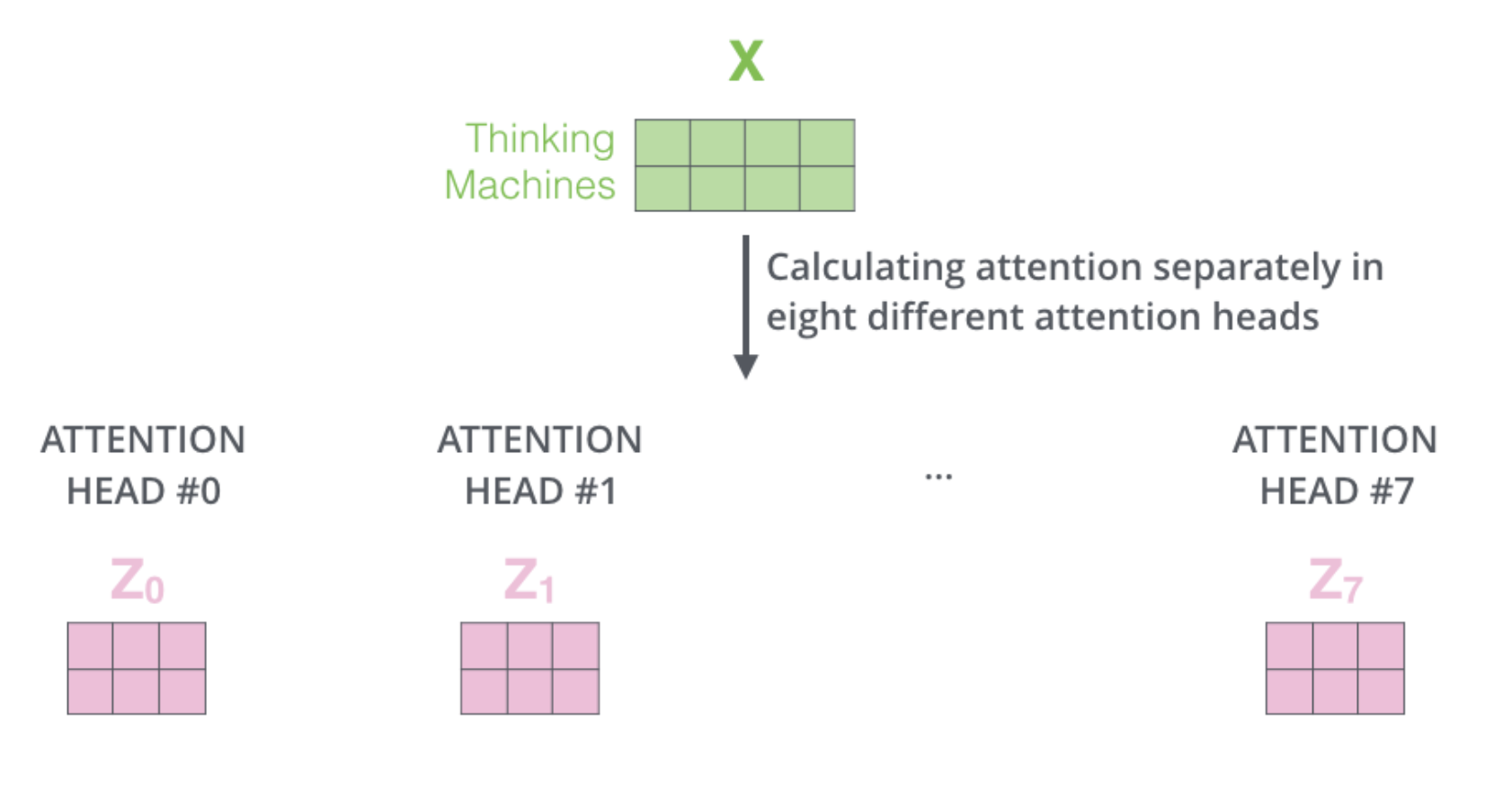
Transformers
Transformers
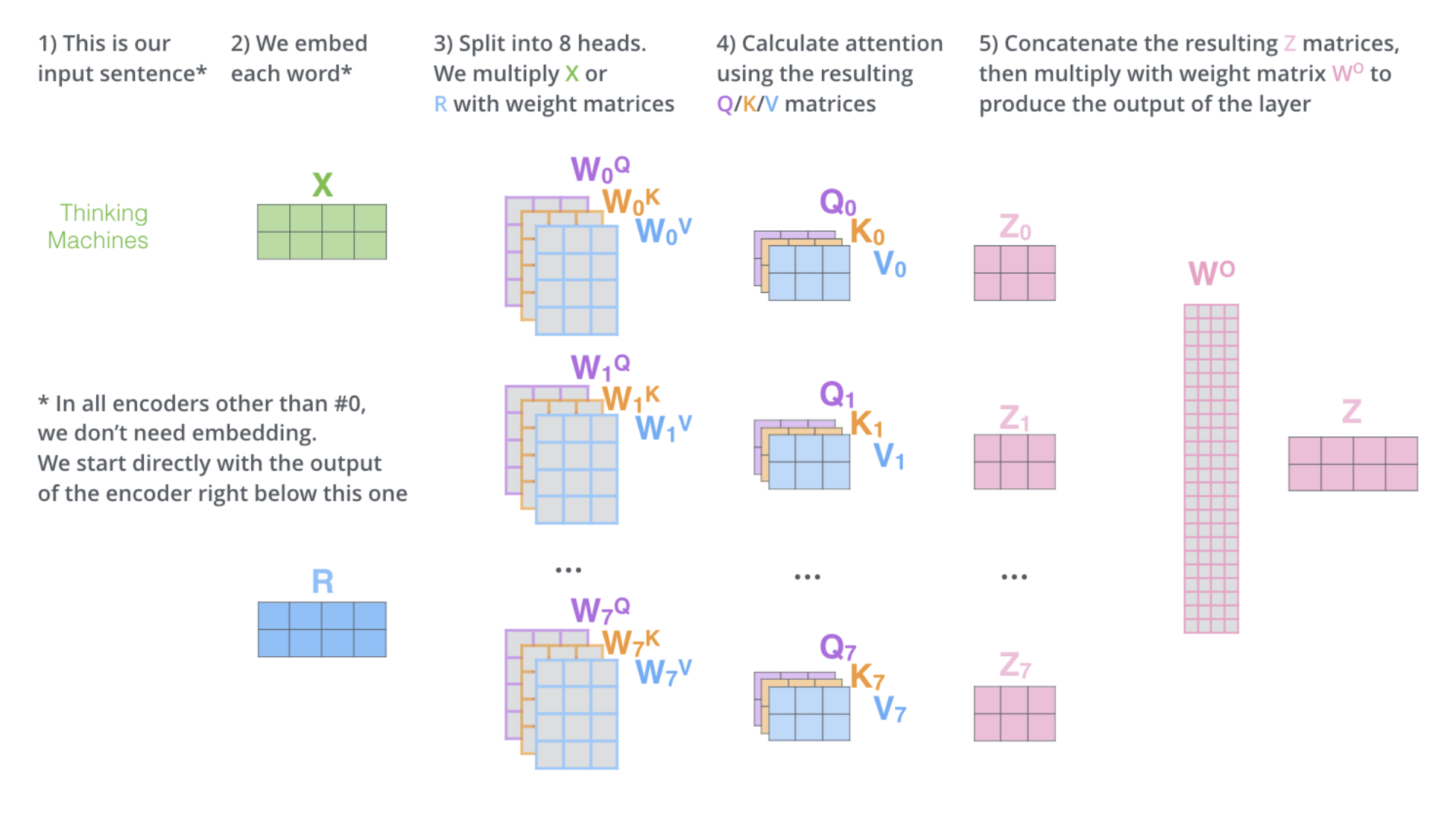
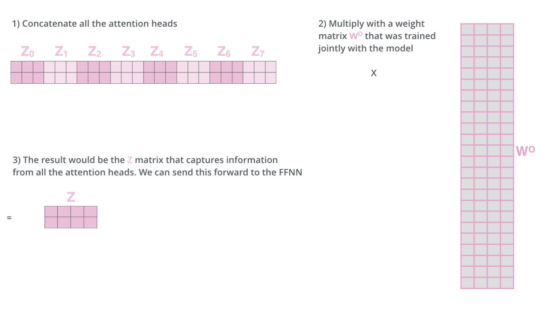
Everything together.
Transformers
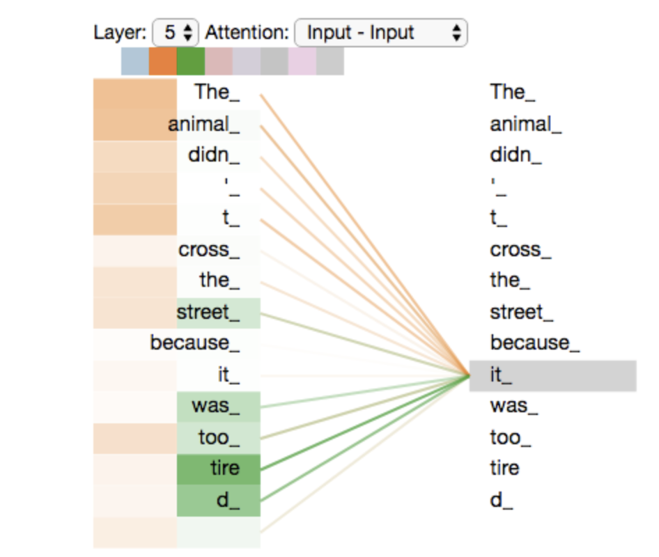
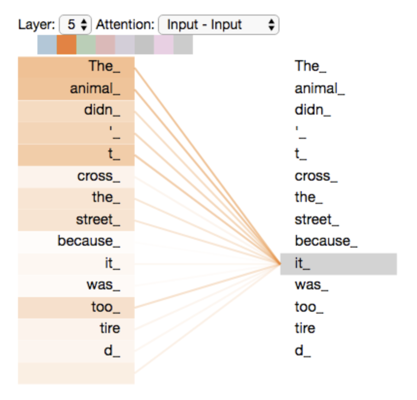
The model’s representation of the word “it” bakes in some of the representation of both “animal” and “tired”.
Transformers
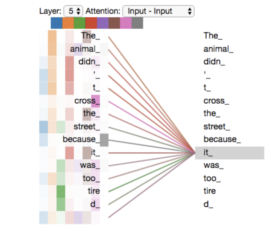
With all attention heads.
Transformers
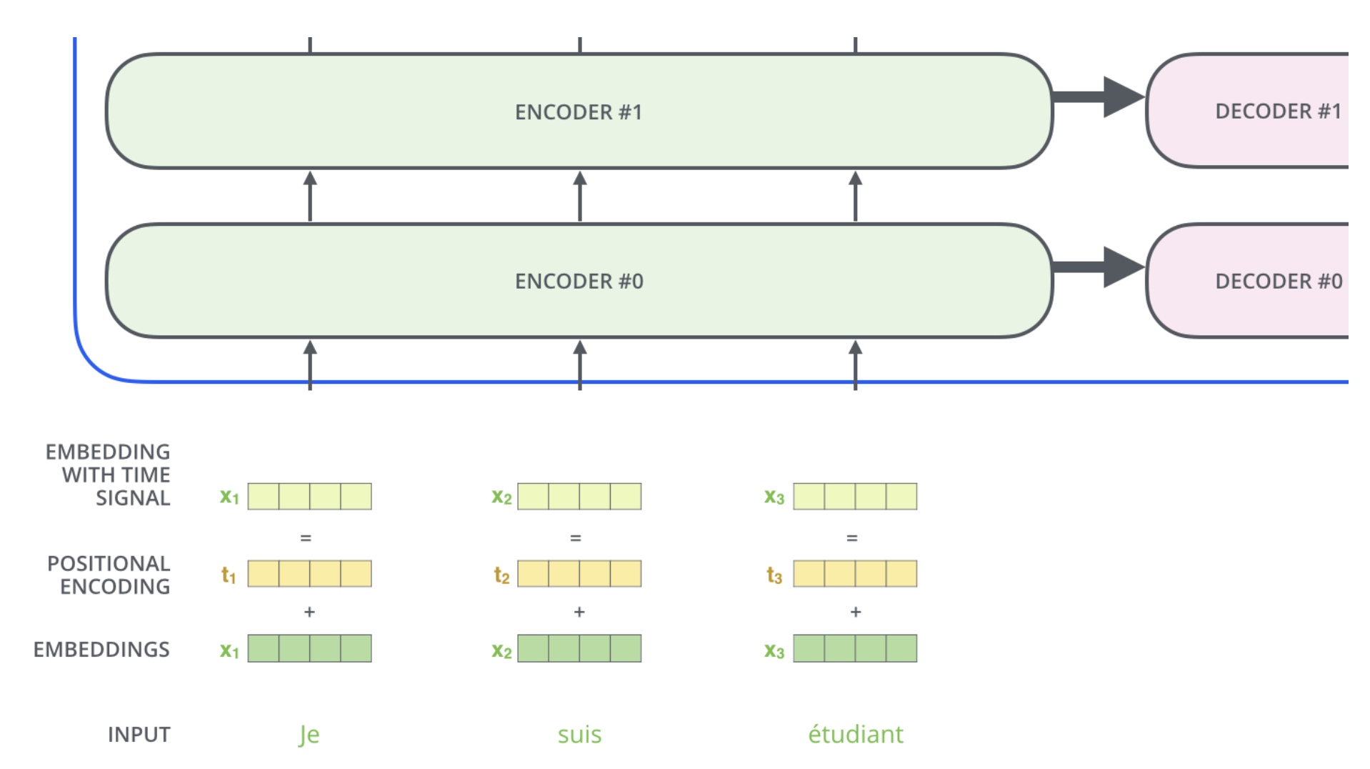
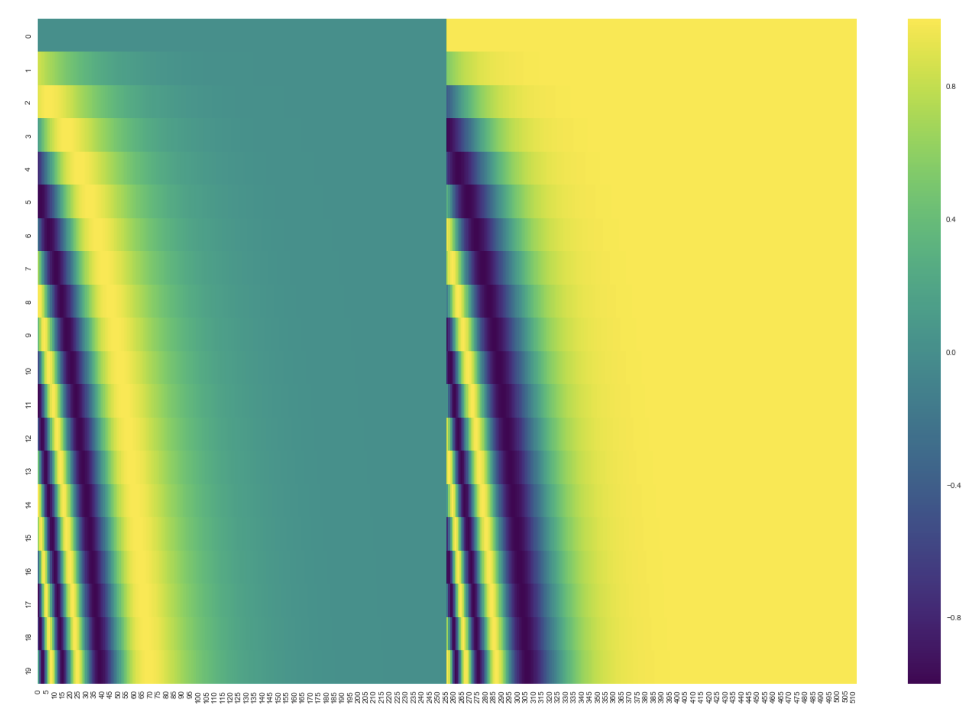
Values of positional encoding vectors follow a specific pattern.
Transformers
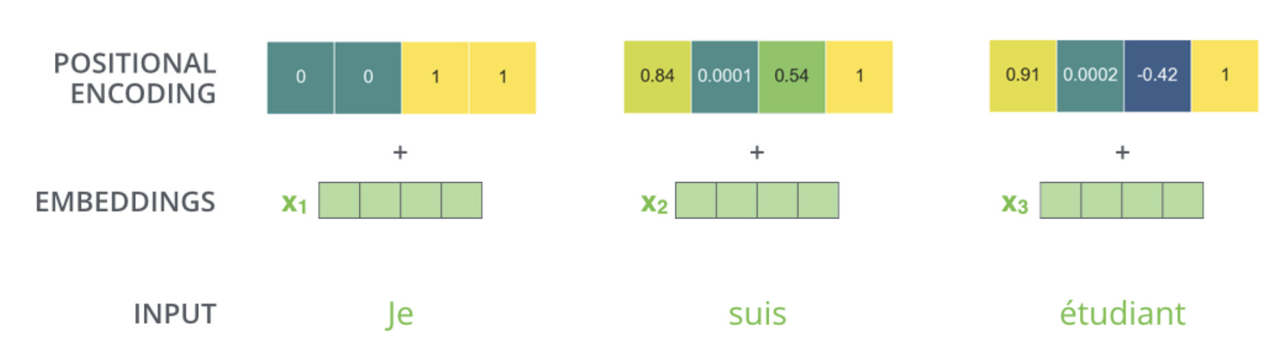
A real example of positional encoding with a toy embedding size of 4.
Transformers
Transformers
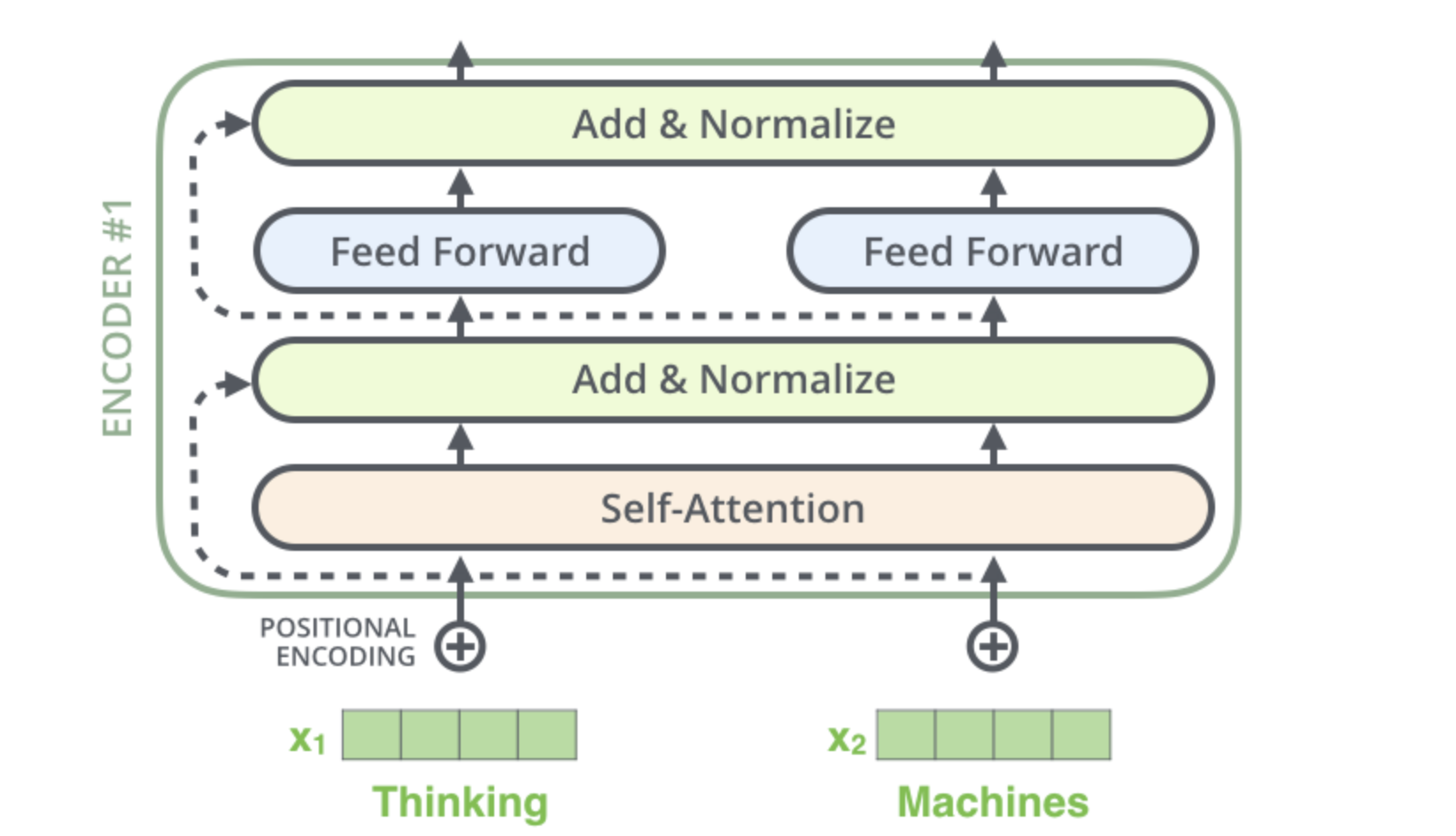
Each sub-layer (self-attention, ffnn) in each encoder has a residual connection around it, and is followed by a layer-normalization step.
Transformers
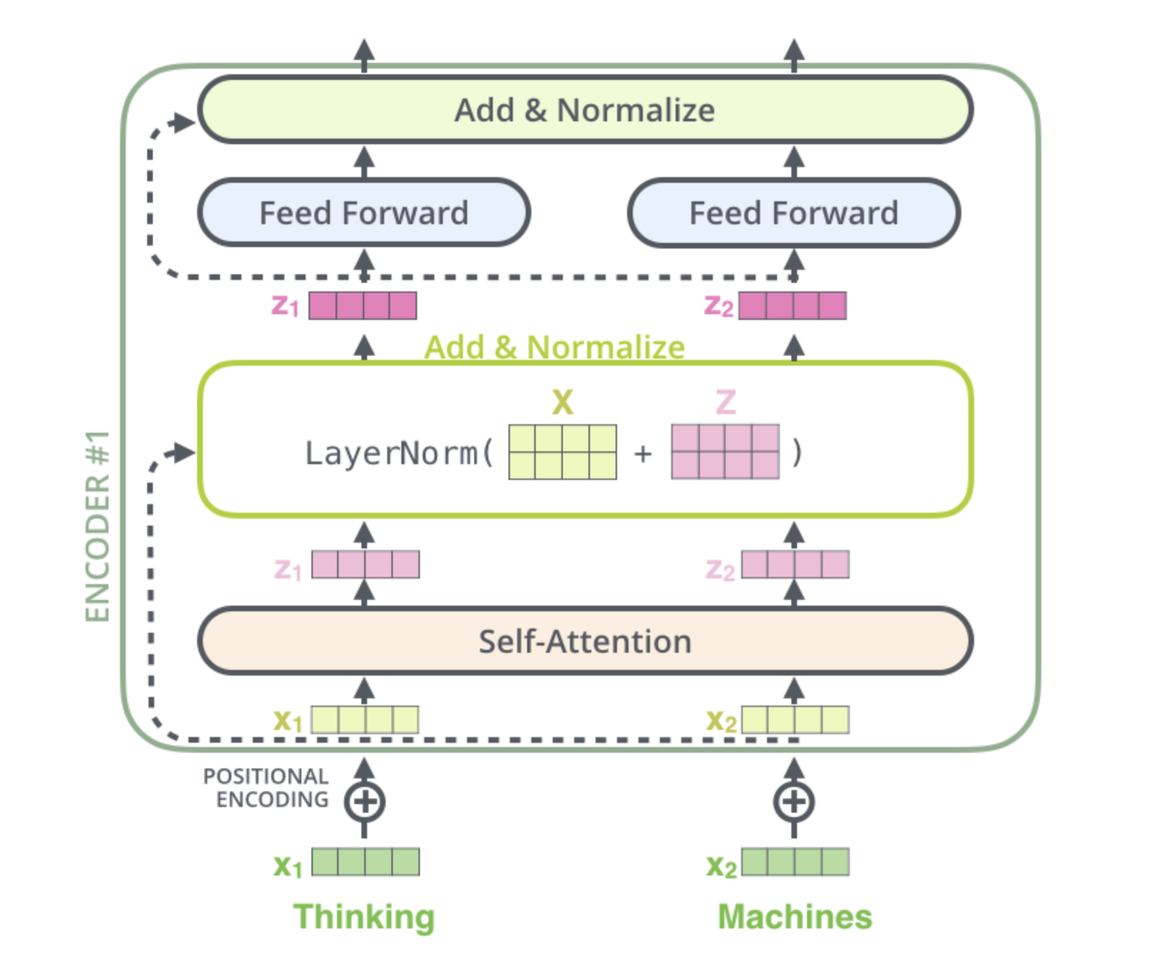
With vectors and operations visualized.
Transformers
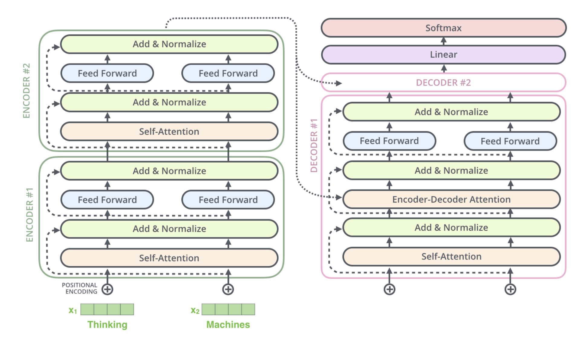
Transformer of 2 stacked encoders and decoders
Transformers
Transformers
Transformers
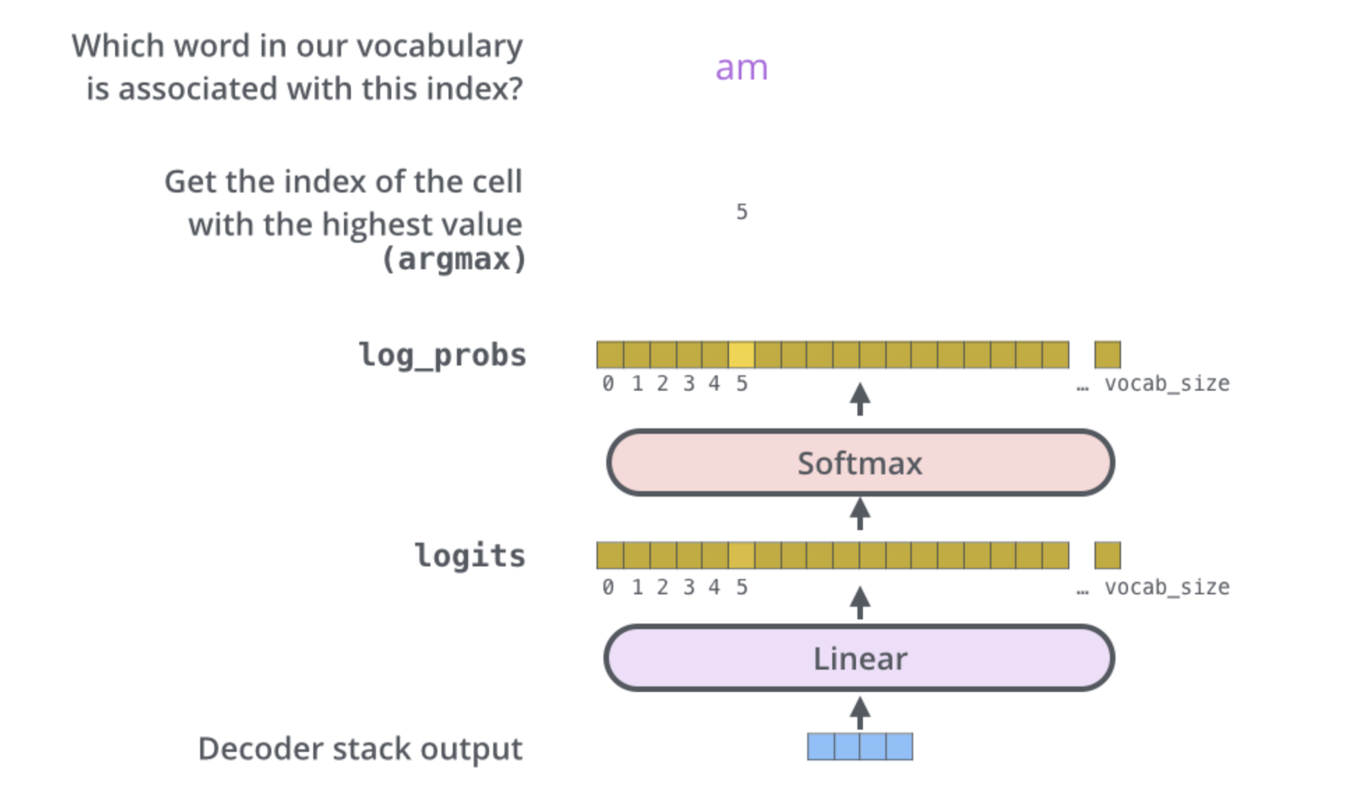
This figure starts from the bottom with the vector produced as the output of the decoder stack. It is then turned into an output word.
Transformers
Training a model
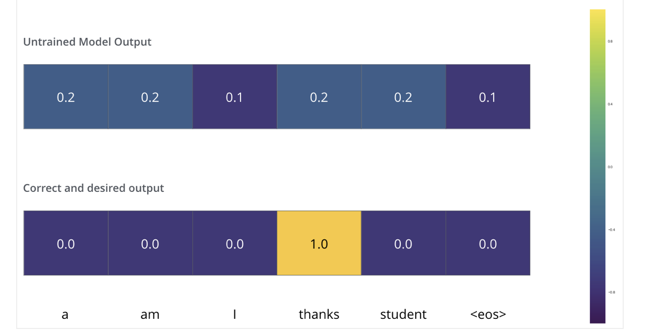
During training, an untrained model would go through the exact same forward pass. But since we are training it on a labeled training dataset, we can compare its output with the actual correct output.
Transformers
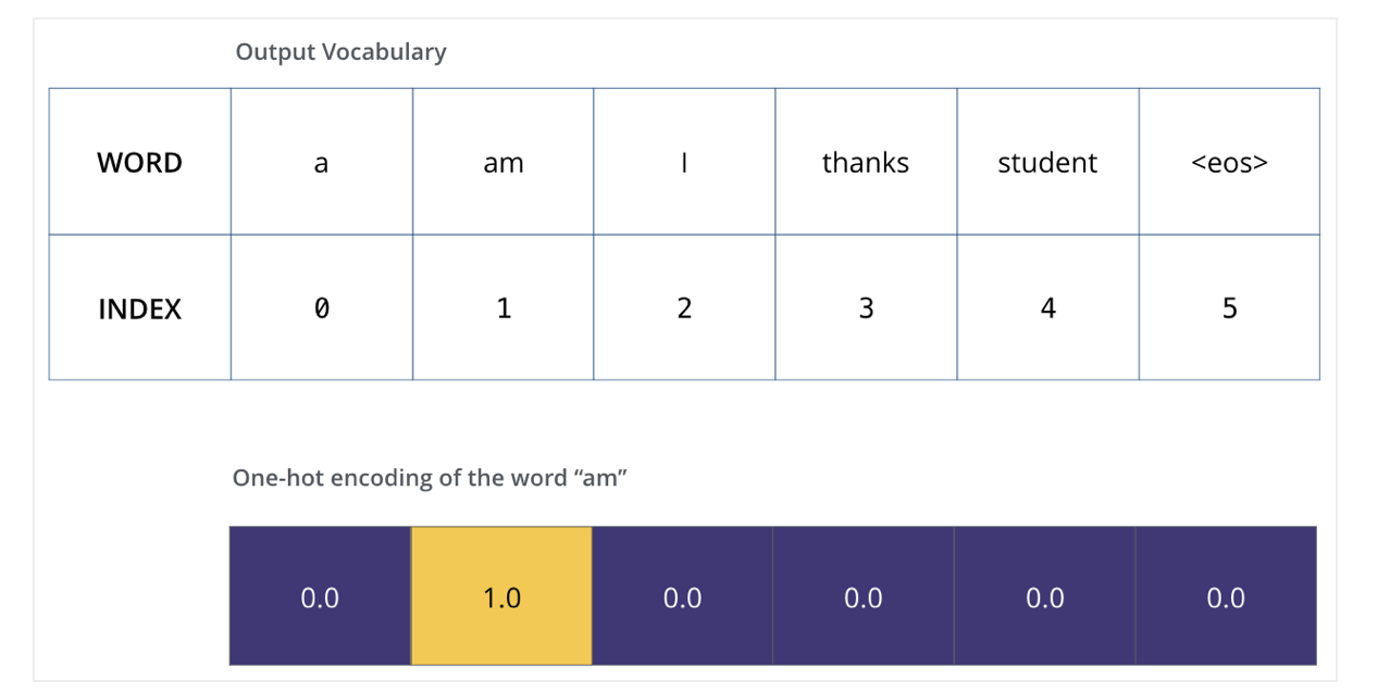
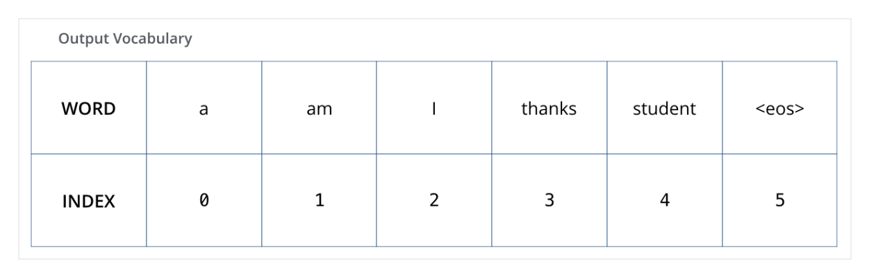
Once we define our output vocabulary, we can use a vector of the same width to indicate each word in our vocabulary. This also known as one-hot encoding. So for example, we can indicate the word “am” using the following vector.
Transformers
The loss function
We want the output to be a probability distribution indicating the word “thanks”.
Transformers
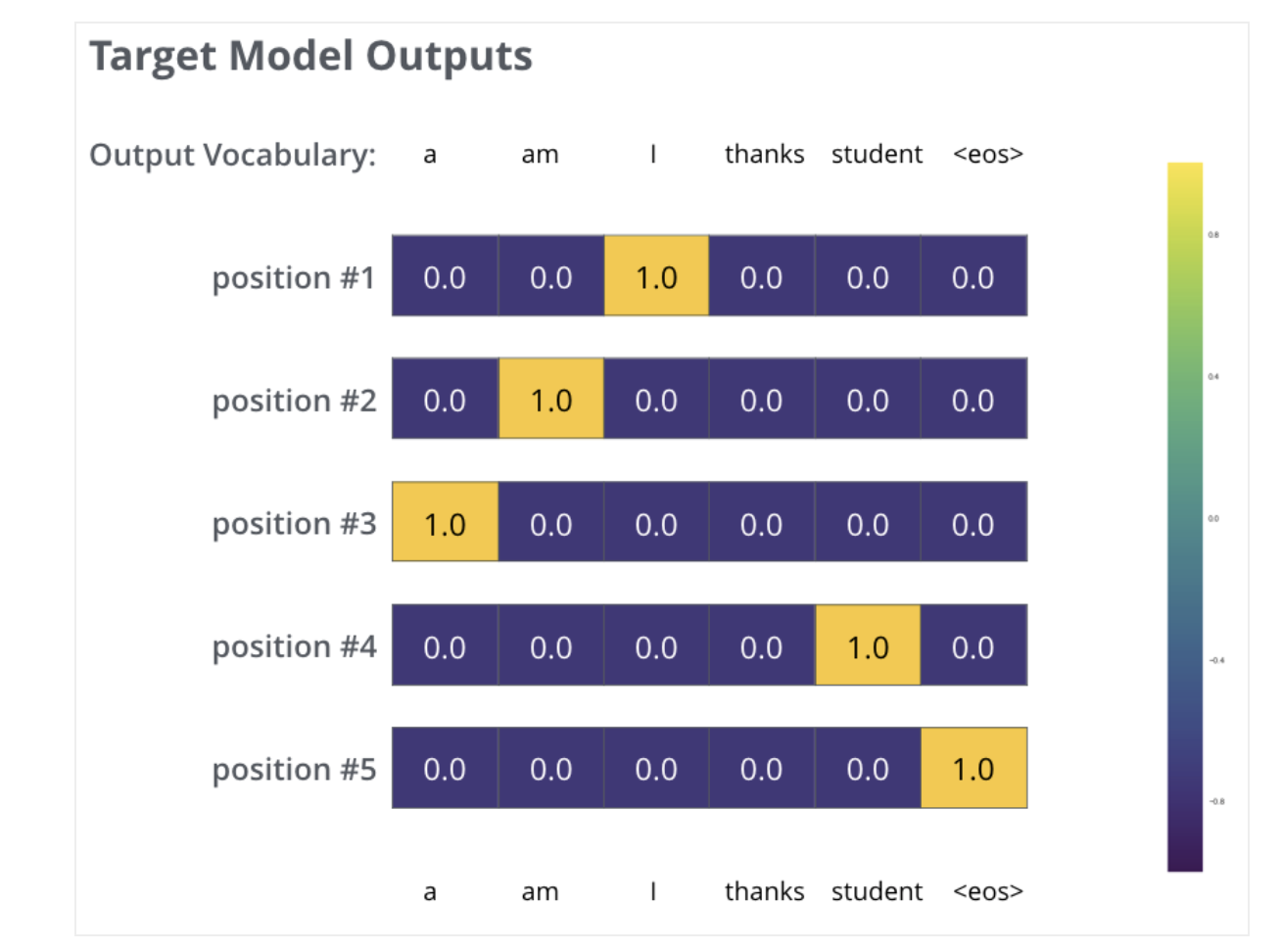
The targeted probability distributions.
Transformers
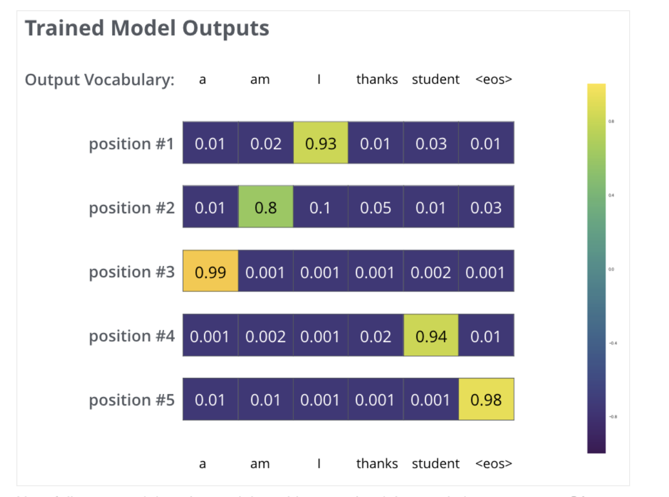
Produced probability distributions.
Attention